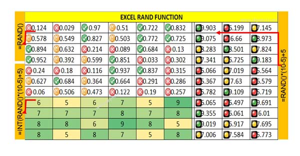
RAND is an important function which is found in Math & Trig category of Microsoft Excel. The Excel RAND function allows you to quickly returns a random number between the 0 and 1 value. With the help of RAND Function you will get a random number which is greater than or equal to 0 and less than to 1, evenly distributed (changes on recalculation).
Also see:
- How to download Voter ID Card in Smartphone
- What is E-PASSPORT, Its FEATURES and How to Apply E-Passport
Must Read: How to use the RANDBETWEEN Function in Excel
If you need to generate a random list when values is between 0 and 1 in that situation Excel RAND function is too much useful for us. RAND Function does not need any argument to generate the random list. After generate the random list, if you press F9 shortcut key then random number list has been changed or recalculated.
Syntax of Excel RAND Function
RAND()
Must Read:
- How to Apply formula on multiple worksheets with 3D reference in Excel
- How to increase Google Chrome speed for suffering and downloading
RAND is the function name which is located in the Excel Math & Trig category. Excel RAND Function allows you to quickly generate a random decimal number list between the 0 and 1.
Step to use Excel RAND Function
RAND Function does not need any argument to generate the random list.

Step 1: Select the cell or range of the cells in which you want to get random number list between 0 and 1.
Step 2: Type =RAND() and press enter without any argument for single cell. If you want to generate random list of more than one cells then you have to drag the result for rest of the cells.
If you already select more than one range of cells then after typing the =RAND() function press CTRL+Enter key to get the result. When you press CTRL+Enter key all the selected range of cells fill by random numbers between 0 and 1.
Always remember if you make any kind of typing or changes random number list has been changed. You can also press F9 function to recalculate the random number list.
Step 3: If you want to generate random number list between two numbers then you have to use given Excel RAND function in active worksheet. In that situation you have to use following formula RAND() * (b – a) + a.
For eg: You want to generate random number list between 5 to 10 then you have to use given function: =RAND()*(10-5)+5 and press enter to get the result.
In this example a is the lowest number while b is the largest number which you want to use to generate a random number list.
Step 4: Excel RAND function generate a random decimal number list between the 0 and 1. But if you don’t want to keep decimal places then you have to use INT function along with RAND function.
=INT(RAND()*(10-5)+5)
Now press enter to get the non decimal random number list as a result.
I hope after reading this guide you can easily understand how to use RAND Function in active worksheet. If you want to become an expert in Excel then you must have to know good command on all the functions. If you have any suggestion regarding this guide then please write us in the comment box.
💬 Loading comments...