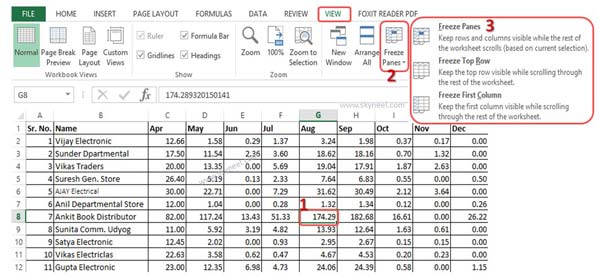
All we know very well about the MS Excel. Lot of time you need to freeze or lock rows and columns in Excel at the same time. I will helps to you easily manage or view large worksheet data from a particular row and a column. There are lot of ways to freeze or lock any row, column as per you need.
Also see:
- How to download Voter ID Card in Smartphone
- What is E-PASSPORT, Its FEATURES and How to Apply E-Passport
Now, if you have a large amount of worksheet data and you want to freeze or lock rows and columns in Microsoft Excel at the same time then you have to read this article. This article helps you to easily understand how to take benefit of freezing or locking facility in MS Excel. There are lot of features available in MS Excel. These features and functions help us to solve any complex problem.
Must Read: How to adding a leading zero value in MS Excel
Freeze panes allows you to lock or freeze any particular portion of the active worksheet which is visible while rest of the part is scrolling. Freeze command is very useful command to check out your large worksheet data.
Lot of time we need to freeze or lock rows and columns in Microsoft Excel at the same time but we don’t know how to do this. This article helps you to easily solve your problem. After that you will be able to easily check out active worksheet data in which particular portion is fixed while rest of the part is scrolling.
Must Read:
How to freeze or lock rows and columns in Excel at the same time:
You have to use following given steps to freeze or lock rows and column in excel. If you want to take benefit of freeze command in Excel then you just have to take following given easy steps:
Step 1: Open an existing large worksheet in which you have number of records.
Step 2: To start freezing process click on the “Freeze Panes” command which is placed in the “View” tab. You can use also use any required option for freezing like Freeze panes, Freeze Top Row and Freeze First Column. These three options available during freezing the row or columns.
If you want to freeze top row only that mean you want to visible top row while rest of the rows are scrolling. Now, you have to select second row in your active worksheet then click on the “View” tab and then click on the “Freeze Top Row” command.
Must Read: Excel: Find Duplicate Values with VLookup in different sheet
You can easily freeze first column only while rest of the columns are scrolling. For this you have to select “B” column in active worksheet. Now, click on the “View” tab and then click on the “Freeze First Column” command.
You can easily freeze or lock rows and columns in Microsoft Excel at the same time. For this you have to select any cell from which you want to start freezing processing. Click on the “View” tab and then click on the “Freeze Panes” command in your active worksheet. Now you will get it will keep rows and columns visible while rest of the part is scrolling.
Note: If you want to unlock rows or columns or remove freeze command effect then you have to click on the “Unfreeze” command which is available in the “View” tab.
I hope after reading this article you will be able to easily freeze or lock rows and columns in Microsoft Excel at the same time. There are lot of interesting and useful commands available in the MS Excel. But freeze command allows you to easily check entire worksheet data in which few part is fixed while rest of the part is scrolling. If you have any suggestion regarding this article then write us in the comment box. Thanks to all.

💬 Loading comments...