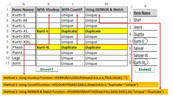
If you have more than one worksheets in the same workbook and want to search duplicate values in two Excel worksheet. It is too much difficult to search duplicate values in Excel sheet. In this guide we have to discuss quick ways which helps you to identifying duplicate values in two Excel worksheet.
It is not so easy to compare two worksheet and search duplicate values in Excel worksheet. If you do this job manually then it will take lot of time to get the result. If you don’t have enough time then you have to use given methods to identifying duplicate values in two Excel worksheets.
- 3 Ways to find duplicate values on same worksheet – Excel
- Get the File Names from a Folder using Excel function
How to Identifying Duplicate Values in two Excel worksheets
Most of the users who are working on the Excel sheet has to face problem during find duplicate values in Excel worksheets. Now, there is no need to worry after reading this guide you can easily search duplicate values in two excel worksheets.

Method 1: Find Duplicate Values in Excel using VLookup function
VLookup function searches a value in the extreme left column of the table_array and provides the value in the same row which is based on the index number.
Syntax of VLookup function: VLookup (lookup_value, table_array, col_index_num, [range])
Note: Before using the VLookup function, first you need to arrange first column of a table or array in the ascending order, otherwise VLookup function is not able to provide the accurate result.
Lookup_value: The value to be searched in the extreme first column of the table array.
Table_array: Two or more columns of data. Give cell reference of a range / range name.
Col_index_num: The column index_number in the table from which the searched value must be returned.
If col_index_num of returns 1 the value in the first column in table_array. If col_index_num is: Less than 1, this function returns an error value the #VALUE!. Sometime it is a greater than the number of columns in table_array, this function returns error value #REF!.
Range_lookup: It is an options part of this function. There are two options available in this part.
TRUE: Appropriate Match: This option work properly when first column of your table will be sorted in ascending order only otherwise it displays wrong
result.
False: Exact Match: VLookup by default check only on exact match method.
Step 1: Fill the given information in two worksheets. Be ensure that both worksheets are exists within a same workbook.
Step 2: Type the following VLookup function in cell K2 =IFERROR(VLOOKUP(Sheet2!A:A,A:A,TRUE,FALSE),”-“). Now press enter to get the result.
Step 3: Drag the VLookup function from K2:K11 to get the result for rest of the cells.
Method 2: Search Duplicate Values in Excel using Countif function
Countif is an important function of Excel. You can easily count all those cells that meet the criteria from given cells values in any worksheet.
Syntax of Countif function: COUNTIF (range, criteria)
range: It is the range of continuous cells which you want to evaluated for the specific condition.
criteria: It is the condition in the form of any number, expression or text value that define which cells to be counted.
Step 1: Type the following given countif function in cell L2 =IF(COUNTIF($A$2:$A$11,Sheet2!A2)=1,”Duplicate”,”Unique”). Now press the enter key to get the result.
Step 2: Now, Select the cell L2 and drag the VLookup function from L2:L11.
Method 3: Identify Duplicate Values using ISERROR and Match function
ISError function is a built-in function in Excel. ISError function is used to checks whether a value is an error (#N/A, #VALUE!,#REF!, #DIV/0!, #NUM!, #NAME?, or #NULL!) and returns True or False.
Syntax of ISERROR: ISERROR (Value)
Value: It is the value you want to test. Value can refer to a cell, formula or a name that refers to a cell, formula or value.
Match function is used to search specific value in the active worksheet. Now this function return the exact position of the value in the given range.
Syntax of Match: MATCH(lookup_value, lookup_array, [match_type])
lookup_value: Lookup values is the value which is search in the table array.
lookup_array: It is the range of cells in which you have to search lookup_value.
match_type: It’s an optional. The default value is 1. The number -1, 0, or 1.
1: Used to find the largest value that is less than or equal to lookup_value.
2: Used to find the first value that is exactly same to lookup_value.
-1: Used to find the smallest value that is greater than or equal to lookup_value.
Step 1: Type the given function in cell M2 =IF(ISERROR(MATCH(Sheet2!A2,$A$2:$A$11,0)),”Unique”,”Duplicate”) and press enter.
Step 2: Again select the cell M2 and drag the function from M2:M11 to get the result for rest of the cells.
It’s not easy to search the duplicate values from large worksheet data. But after reading this guide you can use given quick ways to identifying duplicate values in two Excel worksheets. If you have any suggestion regarding his guide the please write us in the comment box. Thanks to all.
💬 Loading comments...