Slicers in Excel is an important feature which is allows you to quickly filter on multiple items on your active PivotTable report. You can easily insert slicers in active Excel sheet to quickly filter pivot tables to get the exact result as per your criteria.
Before the previous version of Microsoft Excel you can use report filters to filter the Pivot Table reports data. But if you have Excel 2010 or upper version then you can easily filtering your active PivotTable report with the help of Slicers feature in Excel.
Must Read: 3 Ways to find duplicate values on same worksheet – Excel
PivotTable is one of the most important and useful feature of Microsoft Excel. PivotTable allows you to quickly extract required data from selected range of cells. If you want to get better business decisions then you must have to know how to quickly analyze the data. We know it’s not so easy when you have large variety of data.
But PivotTable is an important feature which not only summarize but also analyze, explore and present your data in few clicks. You can also create PivotCharts which is based on the PivotTable. It you made any correction in the PivotTable it will automatically reflect on the PivotChart also.
Slicers in Excel used to Filter PivotTable Data
If you want to use slicers in Excel then first you must have to create a PivotTable to use quickly filtering the PivotTable reports. To use slicers in Excel you must have to take following given simple steps.

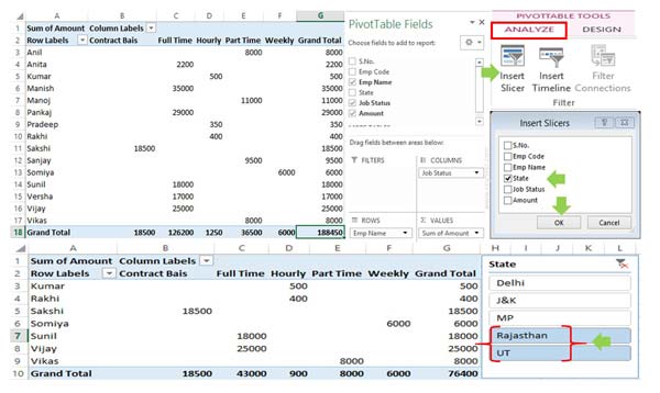
Step 1: Create or active the existing PivotTable. Click on any cells in-side the active Pivot Table.
Step 2: Click on the Insert Slicer option which is located in PivotTable Tools > Analyze tab.
Must Read: How to compare data between two lists in Excel
Step 3: If you want to view State wise reports then turn-on State check mark and click OK button. Click on the particular state which report your want to view. If you want to view more than one state wise report at the same time then you have to hold down Ctrl key and click on the another state name. Now, you can view both active State wise detail in active PivotTable report.
I hope this guide is relay helpful for all those Excel users who are working on the PivotTable and get the summary of large database. After create the PivotTable you can easily summarize, analyze, explore your active PivotTable as per your need. You must have to use slicers in Excel to quickly filter the PivotTable data. If you have any suggestion regarding this article then please write us in the comment box. Thanks to all.
💬 Loading comments...