How to create a simple debt calculator with the help of PPMT Function in MS Excel. We are using three Excel functions PMT, IPMT & PPMT. PPMT stands for Principal Payment of Monthly Instalment. This function is used to calculate how much the amount of principal will be paid with interest amount. You can easily apply PPMT function on all versions of MS Excel.
PMT stand for Payment Monthly Instalment. IPMT stands for Interest Payment Monthly Instalment. PPMT stands for Principal Payment Monthly Instalment. This function is shows the principal amount for a particular payment based on an annual interest rate and a constant payment schedule. In other words, this function will be used to find out how much the amount is paid against the loan.
Syntax of PPMT Function:
PPMT(rate,per,nper,pv,[fv],[type])
rate: Annual Interest Rate
per: Period
nper: Number of Period
pv: Present/Principal Value
fv: Future Value (It will be optional)
type:(It will be optional). It indicates when the payments are due. Type can be one of the following values:If the Type parameter is ignored, then PPMT function supposes that a Type value of 0.
| Value | Explanation |
| 0 | Payments are due at the finish of the period. (default) |
| 1 | Payments are due at the beginning |
For example you want to take loan on four wheeler of Rs. 100000/- at 12.50% annual interest rate for 12 months, in that case you have to take given below following few easy steps to calculate PPMT in any version of Microsoft Excel.
Must Read: Switch /Transpose Row And Column Data in MS Excel
How to use PPMT Function in Excel
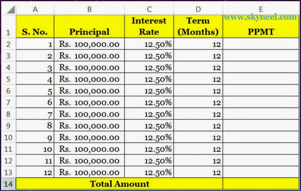
Step 1. Prepare the following sheet in any worksheet of MS Excel.
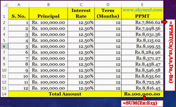
Step 2. Type the following formula in cell E2. You have to divide annual interest rate by 12 to calculate monthly interest rate. =PPMT(C2/12,A2,D2,-B2). When you press enter key, Excel displays the result Rs. 7,866.22/-.
Step 3.Now copy this formula in the following range E3:E13 by dragging mouse button.
Step 4. When you calculate total of all principal amount on the Cell E14 =SUM(E2:E13), Excel displays the result Rs. 1,00,0000/-. It will be same or equal to Principal Amount.
Must Read: How to Restrictions on Columns by Data Validation in Excel
I think you like this post and also sort out your problems. Give your important suggestions in comment box and also share this article with your friends and staff members. Thanks.


💬 Loading comments...