Hi Guys, we know very well about the VLookup function in Excel. VLookup function is widely used at different places to prepare MIS (Management Information System) reports. If you want to search any specific value in the given range of cells or an array during preparing MIS report. Today we discuss how to use VLookup function with two lookup values in Microsoft Excel. The MIS reports are helpful for the top management to take right decision for company growth.
🔥 Trending: How to download Voter ID Card in Smartphone
✅ Must Read: What is E-PASSPORT, Its FEATURES and How to Apply E-Passport
VLookup function with two lookup values in Microsoft Excel
Most of the time when you apply VLookup function only single lookup value is used. Lot of time we need to enter more than one lookup values during using VLookup function. In that situation we will be confused how to use VLookup function with two lookup values in Microsoft Excel. After reading this article your problem will be solved. For novice users first we have to discuss about the VLookup function.
Must Read: Vlookup merge data from one sheet to another Excel worksheet
Definition of VLookup function:
VLookup function is placed in the “Lookup and Reference” category in the Microsoft Excel. VLookup stands for Vertical Lookup. VLookup function is used to search a value in the first column of a table_array or range of cells. After that return corresponding value in the same row and from a column that you specify. First column is always sorted in the ascending order.
Syntax of VLookup function:
VLookup function in MS Excel is search a value in the extreme left column of the table_array and provides the value in the same row which is based on the index number.
= VLookup (lookup_value, table_array, col_index_num, [range])
Note: Before using the VLookup function, first you need to arrange first column of a table or array in the ascending order, otherwise VLookup function is not able to provide the accurate result.
🔥 Trending: How to make voice calls with Reliance Jio from non-VoLTE 4G phone
✅ Must Read: Customize Default Saved Settings in MS Word
Lookup_value: The value to be searched in the extreme first column of the table array.
Table_array: Two or more columns of data. Give cell reference of a range / range name.
Col_index_num: The column index_number in the table from which the searched value must be returned.
If col_index_num of returns 1 the value in the first column in table_array.
If col_index_num is: Less than 1, this function returns an error value the #VALUE!.
If it is a greater than the number of columns in table_array, this function returns error value #REF!.
Range_lookup: It is an options part of this function. There are two options available in this part.
TRUE: Appropriate Match: This option work properly when first column of your table will be sorted in ascending order only otherwise it displays wrong
result.
False: Exact Match: VLookup by default check only on exact match method.
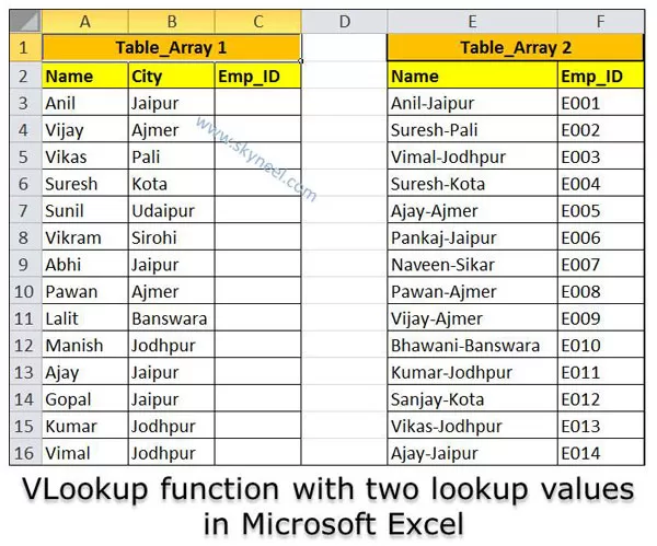
For Eg: If you have two table array and you want to lookup two values in the given table array with the help of VLookup function and get the final result. VLookup function with two lookup values in Microsoft Excel helps you provide accurate result. In that situation you must have to take following given steps..
Must Read: Excel: Find Duplicate Values with VLookup in different sheet
Step 1: If you want to apply VLookup function with two lookup values in Microsoft Excel, first prepare the following worksheet as per given below.
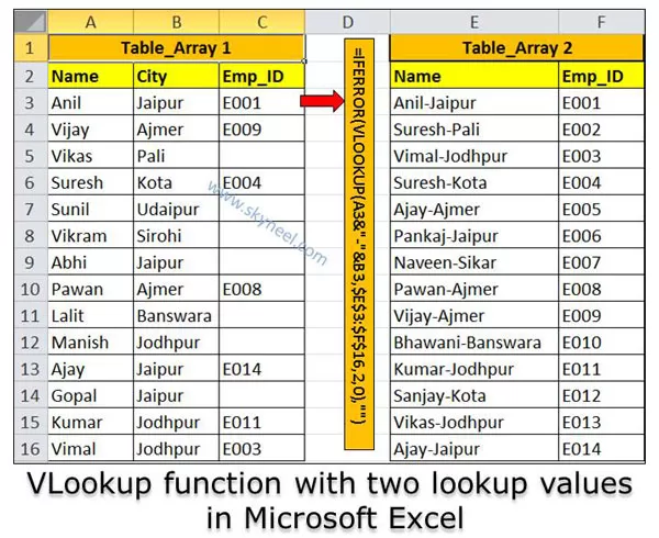
Step 2: Take the cursor on cell C2 and type the following formula to lookup the value.
=IFERROR(VLOOKUP(A3&”-“&B3,$E$3:$F$16,2,0),””)
After typing the formula press enter or return key to get the result.
Note: During selecting the range of Table_array you must have to press F4 function key to change the relative to absolute reference of your Table_array. By default Table_array displays in the relative cell address. With the help of Function key F4 you can easily convert it into absolute or mixed cell reference as per your need.
Ampersand (&): Ampersand operator is a text joining operator which is used to join more than one text strings. In that situation ampersand operator combine name and city along with dash sign.
IFERROR function: IFERROR function is used to check any errors in the formula. This function return a value which you specify when this formula generate any error, otherwise it return the result of the formula.
Step 3: Select the cell C2 and drag the fill handle button from C2 to C16. After releasing the mouse button shows you result in all those cells which match the condition while rest of cells are blanks.
I hope this guide helpful to know how to use VLookup function with two lookup values in Microsoft Excel. This article help you to prepare MIS report with the help of VLookup function. Kindly share this article with others and improve your knowledge. Write your important suggestions regarding this article in the comment box. Thanks to all.


💬 Loading comments...