VLookup is too much popular and important function which is located in Lookup & Reference category. When you want to lookup any value in complex criteria then VLookup is best function or tool to solve your problem. Today we discuss a latest VLookup trick to search with more than one criteria in Excel.
VLookup is used to Looks for a value at the extreme left most column of a table, and return the value in the same row from a column which is specified by you. You have to remember one thing that selected table must be sorted in the Ascending order.
Must Read: Prevent duplicate values with Data Validation in MS Excel
Latest VLookup trick to search with more than one criteria in Excel
There are lot of situations in which you have to use VLookup function in Excel. You can easily use VLookup to search duplicate values in Excel. If you have more than one worksheet then you can easily find duplicate values with VLookup function in different sheet.
You have to use VLookup function in different situations to lookup any value from complex criteria as per your need. In this guide we have to discuss latest VLookup trick to search with more than one criteria in Excel.
For eg: If you have a large worksheet data and want to search about the incentive eligibility and amount which matched the given condition. In that situation you have to use VLookup function with ampersand (&) operator which helps you to search more than one criteria in Excel.
If you have more than one criteria and want to use given latest VLookup trick to search with more than one criteria in Excel then, you have to take few given steps.

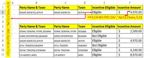
Step 1: Create a new worksheet and fill the given detail in different rows and columns.
Step 2: To set the range name first you have to select the range of cells from B5:F11. Now, click on the Name box and type the “Data” in the name box and press enter.
Must Read: How to find duplicates using conditional formatting in Excel
Step 3: Take cursor on cell E2 and type the given formula to get the Incentive Eligible result: =VLOOKUP(C2&”,”&D2,Data,4,0). If you have more than one criteria then you have to use ampersand “&” operator to join them. Now press enter to get the result.
Note: During typing the formula either you have to type the range name or you can also press F5 shortcut key to quickly open Go To dialog box and select the range name.
Step 4. If you want to calculate Incentive amount then you have to type given formula in cell F2: =VLOOKUP(C2&”,”&D2,Data,5,0). After typing the formula press enter key to get the incentive amount as per matched criteria.
Note: You have to use F4 function key to change the type of reference of any cell.
Finally you can get the Incentive eligibility and incentive amount of that party which match the given criteria.
The latest VLookup trick to search with more than one criteria in Excel article helps you to easily solve your problem. There are lot of situation in which you have to use VLookup function to get the correct result. If you have any query or suggestion regarding this guide then please write us in the comment box. Thanks to all.
💬 Loading comments...