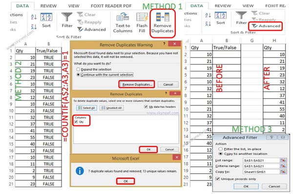
Hi friends, today we discuss about how to find duplicate values from the huge worksheet data in Microsoft Excel, because this problem is faced by many users during doing job in any multinational company or facing interview section. Today we discuss top 3 Ways to quickly find duplicate values in Excel. Here I am provide you a simple way from which you can easily search values which are feed in the given range of cells more than one time. You have to use most popular function “Countif” in Microsoft Excel to quickly find duplicate values from given huge database.
3 Ways to quickly find duplicate values in Excel:
Countif() is a very popular statistical function of MS Excel, which can be used to count numeric values from given range of cells as per match given condition. This article helps you to give simple solutions by writing 3 ways to quickly find duplicate values in Excel. But first we have to know about the countif function in MS Excel. The syntax of this function is given below:
=COUNTIF (RANGE, CRITERIA)
Range: It is a range of non-blank cells, which is used to count number of cells.Criteria: You have to give and specific condition which you want to give as per your requirement to count the number of cells.
For example: If you have a large database and you want to quickly find duplicate values then you have to take following given steps:Type the following values in given range of cells: A1:A22 {Qty, 10, 21, 19, 23, 10, 32, 12, 10, 21, 32, 37, 41, 55, 40, 12, 10, 11, 2, 9, 23}.Type “True / False” in cell B1.
Must Read: Highlight Current Month Birthdays in Excel 2013
Method 1: By using “Remove Duplicates” option from Data Tab:
It is the simplest way to quickly remove all duplicate values from the selected range of cells in MS Excel.
Step 1: Select the range of cells A1:A21.
Step 2: Click “Remove Duplicates” option from Data Tools category in Data Tab.
Step 3: Select Continue with the current selection option > Click on the Remove Duplicates button in Remove Duplicates Warning dialogue box > Click OK button.
Method 2: By using Countif Statistical function:
Step 1: Type the following given formula in cell B2 =COUNTIF (A$2:A3, A3) = 1.
COUNTIF: Statistical Function Name.
A$2:A3: Range of cells. Convert A2 relative cell reference in mixed cell reference by pressing F4 function key after active the formula. A3: Criteria, in which you have to set the condition.
Step 2: After applying this formula in cell b2 you will get the result “TRUE” drag this formula up to B21 cell.
Step 3: Select the range A1:B21 then press CTRL+SHIFT+L to active filter option. You can also click “Filter” command either from Home or Data Tab.
Step 4: Click the drop down arrow of “True / False” in cell B1 and select only “False” category to view all records that match from false condition and remove these record.
Must Read: MS Excel: How to count total “White Spaces” in Text String
Method 3: By using Advance Filter option:
Step 1: Select the range A1:B21 then click on the “Advanced” option from DATA Tab and set the following given condition in “Advanced Filter” dialogue box.
Step 2: Choose “Copy to another location” option and set the range $A$1:$A$21 in List range option. In Copy to line give any cell address where you want to view the result like Sheet1!$H$1.
Step 3: Turn on Unique records only option and finally click on the OK button to get the list of all unique values.
I hope after reading this article you will be able to easily know top 3 Ways to quickly find duplicate values in Excel. if you feel good then please share this article with your friends, colleague.

💬 Loading comments...