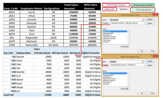
Pivot table is an important and powerful feature of Microsoft Excel. A pivot table allows you to easily arrange and summarize complex data. Sometime you need to create and modify calculated fields in Pivot Table. This feature provide more power to your active pivot table. Pivot table allows you to create or add calculated fields, apply formulas, modify and delete them as per your need.
Must Read: How to Find Duplicates with Pivot Table in Excel
The Calculated filed is very useful and important feature of Pivot table, which allows you to do more calculations on your data to get the required result. You can create your own formula with in a pivot table. You can use this feature to add any new desired field in active pivot table and get the result of fields in your dataset within the pivot table. After applying any calculations which is based on any condition with the help of formula you will get the result in newly added filed. You can apply sum, multiply, count, average, if and other important excel functions in newly added filed. You can also modify or delete them, if required.
A pivot table is especially useful to get summarize the large amounts of data. Pivot tables is one of most powerful features of Microsoft Excel. The pivot table allows you to extract the required data from large amount of data set.
How to create and modify calculated fields in Pivot Table
For example, in the screen shot below, a calculated field, named Bonus, has been created, and it will calculate 3% of the Total, if the sum of Units is greater than 100.

Step 1: Open an worksheet in which you have pivot table. If not then first prepare the pivot table as per your need.
Must Read: How to Show Percentage of Parent Total in an Excel PivotTable
Step 2: Active the pivot table and click on the Analyze > Fields, Items, & Sets option > Click on the Calculated Fields… option.
Step 3: To add the new field you have to set the new field name in the Name box. In the Formula box set the required formula as per your need. After finish this process click on the OK button in Insert Calculated Field box. To get net amount first fill the name “Net Amount” in the Name box. Now, fill the required formula in Formula box. =’Total Sales Amount’ -‘NPD Sales Amount’
Step 4: To add Eligible for incentive new filed column again Insert Calculated Field box. Fill “Incentive” in Name box and type the given formula in Formula box. = IF(‘Total Sales Amount’>=100000,1,0).
Must Read: MS Excel: How to Count values in MIS report PivotTable
How to change format of new calculated fields in Pivot Table
You can also rename inserted new filed name as per your need from pivot table. Now you can check only 1 and 0 is shown in Eligible for Incentive box. You can convert them with “Eligible for Incentive” or “Not Eligible”.
To do this job select the Incentive column in Pivot Table > Press right mouse button.
You have to click on Value Field Settings… > Number Format button > Choose Custom option.
In the Format Cells box > type the following “Eligible for Bonus”;;”Not Eligible” > OK > OK button.
If you want to make any changes in applying formula for new filed or want to delete them, then again open Insert Calculated Field box. Select the new field name in the Name box and make required changes in applying formula as per your need. After done all the changes in the existing formula click on the “Modify” button > Press OK button.
You can also delete any existing new added filed column or formula. To do this job select the filed name and click on the “Delete” button in Insert Calculated Field box.
💬 Loading comments...