PivotTales is one the most important and powerful feature of Microsoft Excel. If you have large worksheet data then you can easily get the summary as per your need with the help of PivotTables in Excel. PivotTables in Excel helps you for quick analysis and take the correct decision for your business.
Also see:
- How to download Voter ID Card in Smartphone
- What is E-PASSPORT, Its FEATURES and How to Apply E-Passport
You can easily analyze, explore and get the summary of required data with in a short period. With the help of PivotTables you can also create PivotCharts also. If you make any kind of modifications in the PivotTable it automatically reflects on the PivotCharts.
There are lot of interesting and useful features of Microsoft Excel. You can use different types of functions, What-If-Analysis, Filter, Conditional Formatting, Data Validation, PivotTables and PivotCharts and many more. All these things increase the popularity of the Microsoft Excel. If you have better control on these feature on Excel then you will become an Excel expert.
Must Read: Important Shortcut keys of Microsoft Excel
PivotTables in Excel Used to Analyze, Summarize Worksheet Data
PivotTables allows you to quickly summarize and arrange large and complex data. You can set different columns detail in the PivotTable structure as per your need. You can also use different inbuilt PivotTables structures from the “Recommended PivotTable” option. To create the PivotTables you must have to take following given steps, have a look.
Must Read:
- How to add proxy setting in Firefox and Chrome for internet
- Improve Camera Quality with Jelly Bean 4.2 Camera and Gallery

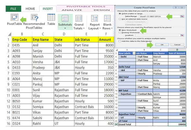
Step 1: Create the following structure or open an existing worksheet in which you have number of records. Select the complete range of cells to create the PivotTables in Excel for analysis and get the summary detail.
Step 2: Click on the Insert Tab > Choose PivotTable option. By default it automatically take the range as per your selection you can also edit the selected range as per your need from Select a table or range option.
Step 3: If you want to create and show PivotTable on new worksheet then choose “New Worksheet” option. If you want to create and show the PivotTable on active worksheet then you have to choose “Existing Worksheet” option. Now, click on the OK button.
Must Read: Beauty of Goal Seek feature in Excel to Find the Answer
Step 4: You can choose or add required columns with your PivotTables. You can also change the active PivotTable settings as per your need. When you active your PivotTable two new tabs are shown in-front of your namely Analyze and Design. Analyze tab allows you to set the PivotTable name, Insert Slicer, Change data source, move, select, clear PivotTable and also insert the PivotChart. Design tab allows you to turn on or off subtotals, grand totals, change report layout and styles as per your need.
I hope after reading this guide you can easily create PivotTables in Excel. You can get the summary of large worksheet data, analysis the data and take the correct decision for your business. If you have any suggestion regarding this guide then please write us in the comment box. Thanks to all.
💬 Loading comments...