Conditional Formatting in Excel is used to change all formatting, background colors, border and shading, and many more as per given condition. In this article we know how you easily change each column background color using conditional formatting facility in excel.
For example for Changing Column Background Color:
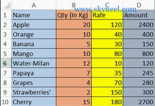
If Column A value is equal to Names then entire column should have a blue background.If Column B value is equal to Qty then entire column should have a light orange background.If Column C value is equal to Rate then entire column should have a yellow background.If Column D value is equal to Amount then entire column should have a gray background.
Must Read: Conditional Formatting How to generate chess board on excel
In this type of condition you have to use following steps given below in excel:
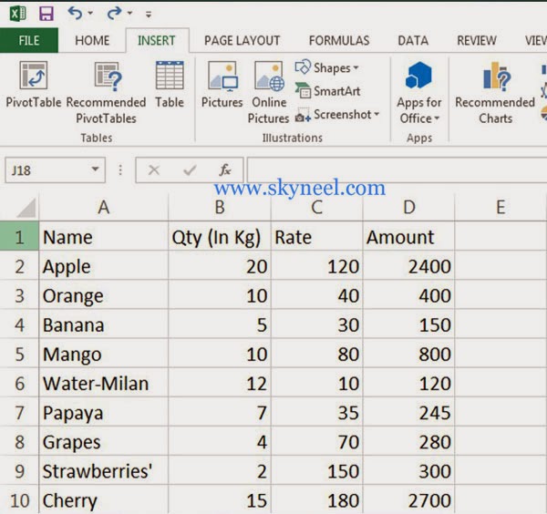
1. Prepare the following sheet only fill required data in each column.
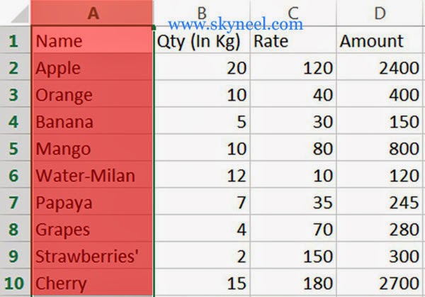
2. Select first column A by clicking column label A.
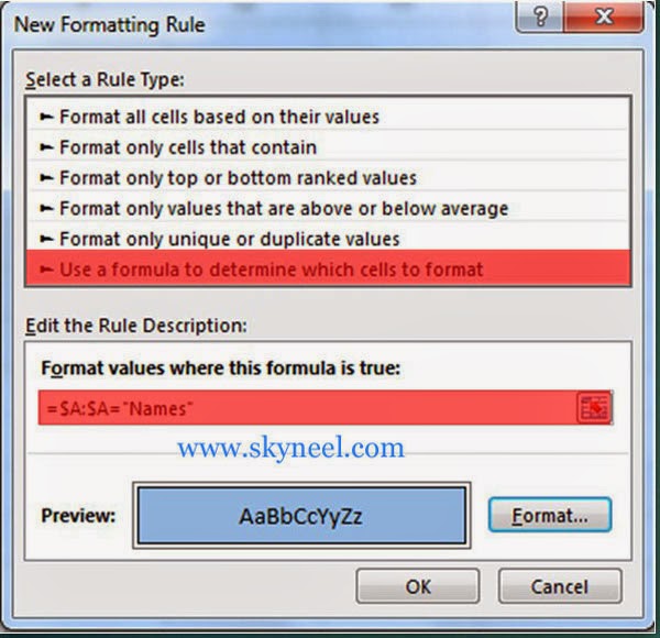
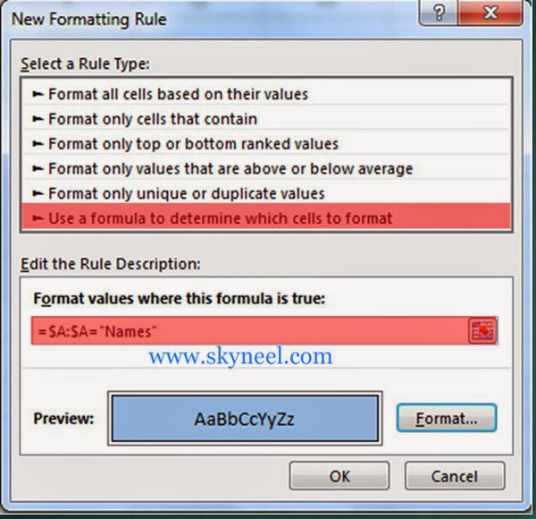
3. Click Home > Conditional Formatting > New Rule > Select a rule type > Use a formula to determine which cells to format > type following formula in given box =$A:$A=”Name” > Click Format button > Fill any required color from fill tab then click OK > Ok.
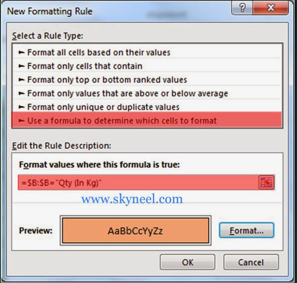
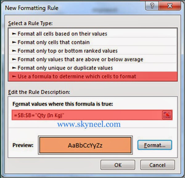
4. Select column B by clicking its column label then click Home > Conditional Formatting > New Rule > Select a rule type > Use a formula to determine which cells to format > type following formula in given box =$B:$B=”Qty (In Kg)” > Click Format button > Fill any required color from fill tab then click OK > OK.
5. Select column C by clicking its column label then click Home > Conditional Formatting > New Rule > Select a rule type > Use a formula to determine which cells to format > type following formula in given box =$C:$C=”Rate” > Click Format button > Fill any required color from fill tab then click OK > OK.
6. Select column D by clicking it’s column label then click Home > Conditional Formatting > New Rule > Select a rule type > Use a formula to determine which cells to format > type following formula in given box =$D:$D=”Amount” > Click Format button > Fill any required color from fill tab then click OK > OK.
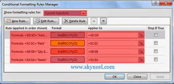
7. To view all column label conditional formatting in conditional formatting manager box by click Home > Conditional Formatting > Manage Rules
8. Result of conditional formatting on each column is given below:
Must Read: Conditional Formatting : Only Text Entries in Excel
I hope you like this Conditional Formatting : Changing Column Background Color guide from which you will be able to easily Changing Column Background Color without any extra efforts. If feel any problem in this guide then please use comment box. Thanks to all.
💬 Loading comments...