Hi Friends, today we talk about Excel conditional formatting to highlighted Weekends in Excel. In most of the companies where 5 days are working days. You can use this post to highlight weekend dates. In excel you can use following given formula in conditional formatting to highlight the rows which dates are Saturday and Sunday.
Must Read: Conditional Formatting : Only Numeric Values in Excel
Meaning of Conditional Formatting:
If you want to apply different formatting features like applying any font, change font color, size and style, draw border and shading on selected one cell or range of cells that match the condition as you specified in active sheet is known as “Conditional Formatting”. It is an important command of MS Excel, from which you can easily and quickly applying formatting effects that match the condition.
How to Highlighted Weekends in Excel:
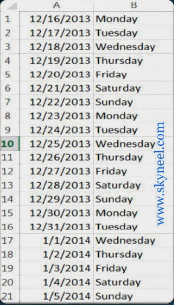
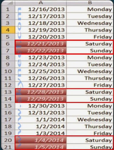
Step 1. Prepare following sheet as per given below, type following dates in range A1:A21 and name of weeks in range B1:B21 like given below:
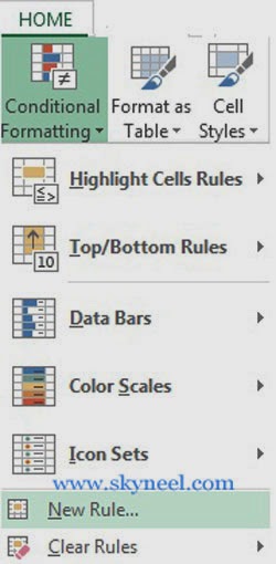
Step 2. Now you have to click on the Home Tab -> Click on the “Conditional Formatting’ feature from the “Styles” group -> Click on the “New Rule” option.
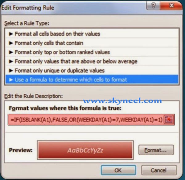
Step 3. Select “Use a formula to determine which cells to format” in Select a Rule Type category. Type the following formula in the Format Values where this formula is true box: =IF(ISBLANK(A1),FALSE,OR(WEEKDAY(A1)=7,WEEKDAY(A1)=1))
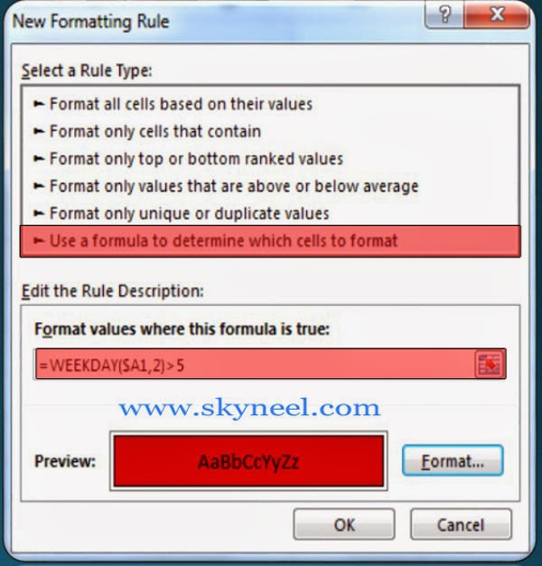
Or, You can also type another given formula for highlighted weekends in conditional formatting in excel:=WEEKDAY($A1,2)>5
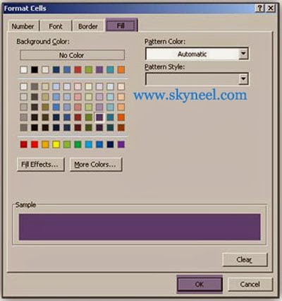
Step 4. Now, you have to click on the “Format” button -> click on the “Fill” button-> Select any color, border and shading which you want to fill then click OK button.
5. Click OK button again to view the result of conditional formatting on selected range of cells.
Note: You can also remove conditional formatting from selected range of cells or entire sheet by clicking on the Home tab -> Click on the “Conditional Formatting” from “Styles” group -> Click on the “Clear Rules” option -> Click on the “Clear Rules from Selected Cells” or you can also click on the “Clear Rules from Entire Sheet” option.
Must Read: MS Excel :Vlookup Function with a Spreadsheet
I hope you like this post. Give your important suggestion in the comment box and also share this article with your friends to show your knowledge in excel. Thanks.
💬 Loading comments...