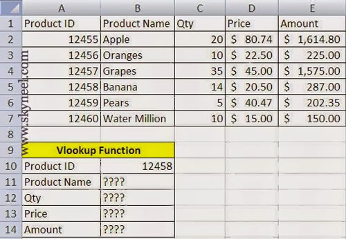
Vlookup function is one of the most powerful and strongly used look-up & reference function of Microsoft Excel. Vlookup is a function that permit you to feed the value of one cell to search the value of a matching cell in the same row. Excel’s VLOOKUP function, “V” stands for Vertical, this function can help you to find exact information in huge data tables just like a stock list or a huge telephone list.
Syntax of Vlookup:
The Microsoft Excel VLOOKUP function search a value in the extreme left column of the table_array and provide the value in the same row which is based on the index_number. =VLOOKUP(lookup_value, table_array, col_index_num, [range])
Note: Before using the Vlookup function, first you need to arrange first column of table or array in the ascending order, otherwise VLOOKUP function is not able to provide the accurate result.
Lookup_value: The value to be searched in the extreme first column of the table array. Table_array: Two or more columns of data. Give cell reference of a range / range name. Col_index_num: The column index_number in the table from which the searched value must be returned.
If col_index_num of returns 1 the value in the first column in table_array.
If col_index_num is: Less than 1, this function returns an error value the #VALUE!.
If it is a greater than the number of columns in table_array, this function returns error value #REF!.
Range_lookup: It is an options part of this function. We have an example how to use “Vlookup” function in excel to find values. This example find the Product ID column of a fruits in the “Products” table and check the values in the Product Name, Qty, Rate & Amount columns to test conditions.
Must Read: Effortless Hindi Typing – Special Character Code
Steps to get the result using Vlookup Function:
1. Prepare the following sheet.
2. Take cursor on Cell B11 to type following formula: =VLOOKUP($B$10,$A$1:$E$7,2,FALSE)
Note: You have to change the cell reference of B10 and range A1:E7 in absolute cell reference by pressing F4 function key, because both are constant during copy and paste this formula on other cells -> Press enter to view the result.
3. Now copy Cell B11 formula in B12 to B14 but change the column_index_number in each formula like given below: Cell B12: =VLOOKUP($B$10,$A$1:$E$7,3,FALSE) Shows Qty of lookup valueCell B13:
=VLOOKUP($B$10,$A$1:$E$7,4,FALSE) Shows Rate of lookup valueCell B14:
=VLOOKUP($B$10,$A$1:$E$7,5,FALSE) Shows Amount of lookup value
Must Read: Excel Formula RANK: Tips to Get Ranking Position
I hope you like this post. Give your important suggestion in the comment box and also share this article with your friends to show your knowledge in excel. Thanks.

💬 Loading comments...