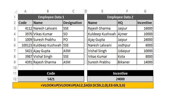
If you have data in two different table or worksheet then you need to apply double VLookup in Excel. At this situation most the Excel user face lot of issue how to get the exact result which match the condition. This article helps you to know how to use Excel Double VLookup function in active worksheet.
💡 You might like: How to download Voter ID Card in Smartphone
👉 Don't miss: What is E-PASSPORT, Its FEATURES and How to Apply E-Passport
Syntax of VLookup function in Excel
Microsoft Excel VLookup function is used to search specific value in the extreme left column of the table_array. This function provide the value in the same row which is based on the index number.
Must Read: How to Search Duplicate Values with VLookup function
VLookup (lookup_value, table_array, col_index_num, [range])
👉 Don't miss: How to watch YouTube videos without Wi-Fi or data
🔥 Trending: How to get Lockdown E-Pass for Covid-19 Lockdown
This function is used to search the value of extreme left column.
Lookup value is used to search in the extreme first column of the table array.You can give cell reference of a range or range name.
Col index num is the column number in the table from which the searched value must be returned.
Range lookup is an options part of this function. There are two options available in this part.
If range is TRUE then it will act just like appropriate match.
When you Set Zero or False i.e. exact match. VLookup function by default check only on exact match method.
How to use Double VLookup in Excel
Must Read: Reverse VLookup in Excel with VLookup Function
If you want to apply double VLookup in Excel sheet then you have to use given simple steps, have a look.

Step 1: Create the following both table either in single worksheet or other worksheet.
Step 2: If you want to to find incentive amount from second worksheet of any specific employee which code matched in first worksheet. In that situation you must have to apply given VLookup function in Excel worksheet.
=VLOOKUP(VLOOKUP(A12,$A$3:$C$9,2,0),E3:G9,3,0)
Now, press enter key to get the result.
I hope after reading this guide you can easily apply double VLookup function in Excel. If you have any suggestion regarding this guide then please let me know via comment box.
💬 Loading comments...