Hi guys, we know very well about the MS Excel. MS Excel is an application software which is widely used in different locations. MS Excel is an electronic spreadsheet software which is used for data analysis, modeling, representation data inform of chart, solve complex calculations using functions and many more. Today we have to discuss VLookup Function in MS Excel with Appropriate Match. It is another very important topic which you face when you go for interview. During doing job in any company or facing the questions about “VLookup” during the interview session. You know very well about the “VLookup”. It is one of the most important functions which is found in “Lookup and Reference” category of Microsoft Excel. There are lot of different examples of VLookup function in MS Excel, which you can use in different situation. Today we have to discuss to search in a spreadsheet using VLookup Function in MS Excel with Appropriate Match.
Also see:
- How to download Voter ID Card in Smartphone
- What is E-PASSPORT, Its FEATURES and How to Apply E-Passport
Must Read: How to use IFNA with VLookup function
When we are using “VLookup” function, most of the cases we use “Exact Match” method in MS Excel. Today I try to tell you how to use VLookup function with “Appropriate Match” in range lookup. VLookup: This function is found in the “Lookup and Reference” categories of Microsoft Excel. So have a look and take few easy steps to use VLookup Function in MS Excel with Appropriate Match:
Syntax of VLookup:
The VLookup function in MS Excel searches a value in the extreme left column of the table_array and provides the value in the same row which is based on the index number.
= VLookup (lookup_value, table_array, col_index_num, [range])
Must Read:
- How to unlock bootloader Google Pixel XL Smartphone
- How to use Excel INT Function to Remove Decimal Places
Note: Before using the VLookup function, first you need to arrange first column of a table or array in the ascending order, otherwise VLookup function is not able to provide the accurate result.
Lookup_value: The value to be searched in the extreme first column of the table array.
Table_array: Two or more columns of data. Give cell reference of a range / range name.
Col_index_num: The column index_number in the table from which the searched value must be returned.
If col_index_num of returns 1 the value in the first column in table_array.
If col_index_num is: Less than 1, this function returns an error value the #VALUE!.
If it is a greater than the number of columns in table_array, this function returns error value #REF!.
Range_lookup: It is an options part of this function. There are two options available in this part.
TRUE: Appropriate Match: This option work properly when first column of your table will be sorted in ascending order only otherwise it displays wrong result.
False: Exact Match: VLookup by default check only on exact match method.
Steps how to use VLookup Function in MS Excel with Appropriate Match:
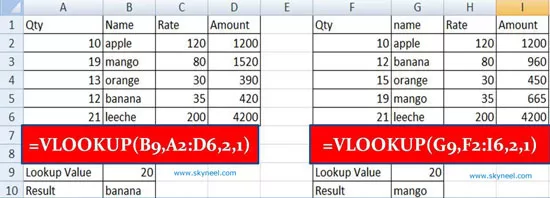
For example, Have a look and find what the main difference when you use “Appropriate Match” option during applying VLookup formula in any sorted and unsorted table.
Step 1: Create the following given table to use VLookup Function in MS Excel with Appropriate Match.

Step 2: Select and copy the range A1:D6 and paste it on F1:I6.
Step 3: Select the range A1:D6 and set the name “Unsorted table” from name box.
Step 4: Select the range F1:I6 and click Home tab > Click “Sort and Filter” option in Editing group > Click Sort A to Z. You can also click Data tab > Click “Sort A to Z” button. Click on the name box and set the name “Sorted Table”.
Step 5: If you want to view the result on unsorted table apply the following given formula on cell B10: =VLOOKUP(B9,A2:D6,2,1). When you press enter, Microsoft Excel displays “Banana” as a result.
Step 6: If you want to view the result on sorted table apply the following given formula on cell G10: = =VLOOKUP(G9,F2:I6,2,1). When you press enter, Microsoft Excel displays “Mango” as a result.

So this is the main difference. When you apply VLookup function on unsorted table Microsoft Excel display “Banana”. While you apply VLookup function on sorted table Microsoft Excel displays “Mango” as a result.
Must Read: Reverse VLookup in Excel with VLookup Function
I hope you like this article. After reading this article you will be able to easily use VLookup Function in MS Excel with Appropriate Match. If you have any query then type your question regarding this post in the comment box. Thanks.
💬 Loading comments...