Lot of time many peoples and confused and face problems during to search any particular value or bring data from one sheet or workbook or a huge database to another sheet or workbook in excel. So, in this article we try to solve your problem to easily search particular values using VLookup and HLookup functions in Excel which is belong to lookup and reference category of MS Excel. These functions are very popular and mostly used by the different users in different fields like finance, bank, accounts, education, construction, and many more fields.
Vlookup and Hlookup Functions in Excel
Let’s take an example from which you can easily understand how to use both functions: Suppose if you have a database of your customer’s quarterly accounts report in which you have your customers account number, customer name, type of accounts and closing balance, now if you want to search any valid account number then the respective details like customer’s name, account type and closing balance will appears automatically. To do this job, you must need to use Vlookup and Hlookup functions.
Must Read: VLOOKUP Compare values in another Excel worksheet
Vlookup Function ():
The Vlookup stands for “Vertical lookup” function which will search for a value in the first column of a table or range of cells and then return corresponding value in the same row and from a column that you specify. First column is sorted in ascending order.
Syntax: =VLOOKUP (lookup_value, table_array, col_index_num, range_lookup)
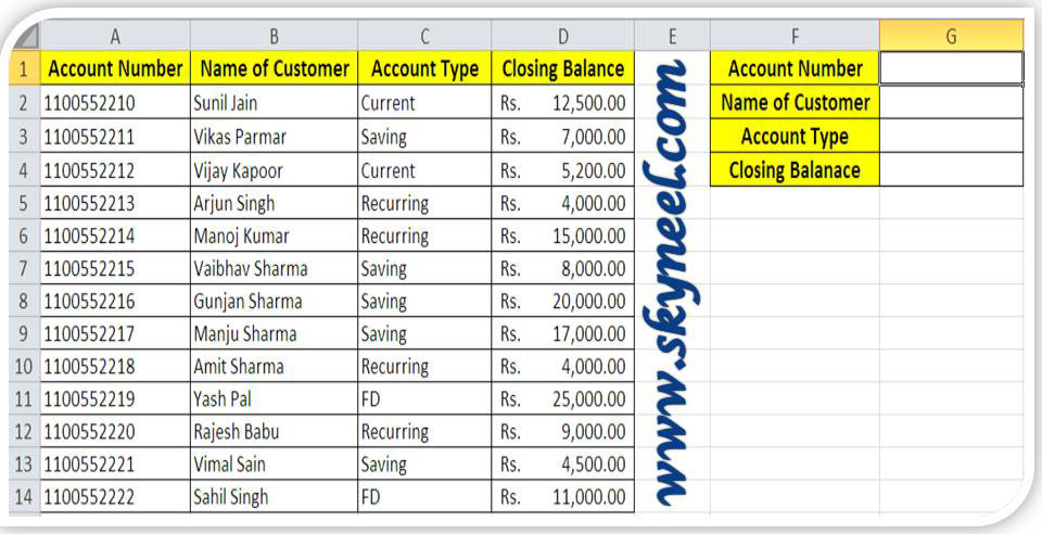
Step 1: Prepare the following given database in excel sheet.
Step 2: To view the customer name take cursor on cell G2 and type the following given formula: =VLOOKUP(G1,A2:D14,2,0).When you press enter, excel displays an error message #N/A. Because you don’t fill account number of the customer in the cell G1.
Note: If you want to copy this formula you must need to change the relative reference type of G1, A2:D14 into absolute reference type by pressing F4 function key. After converting them in to absolute reference type, formula looks like: =VLOOKUP($G$1,$A$2:$D$14,2,0)
Step 3: To view the customer account type take cursor on cell G3 and type the following given formula or you can also copy formula from cell G2 and change the col_index_number like this: =VLOOKUP($G$1,$A$2:$D$14,3,0)
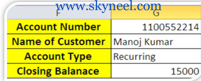
Step 4: To view the customer closing balance take cursor on cell G4 and type the following given formula or you can also copy formula from cell G2 and change the col_index_number like this: =VLOOKUP($G$1,$A$2:$D$14,4,0). After applying the formula it shows following result.
Note: After applying all formulas, insert account number of any customer in cell G1, excel automatically displays values of all cells.
Hlookup Function ():
The Hlookup stands for “Horizontal lookup” function which is used to search for a value in the top row of a given table or array of values and return the corresponding value from the same column in a row that you specify.
Syntax:
=HLOOKUP (lookup_value, table_array, row_index_num, range_lookup)
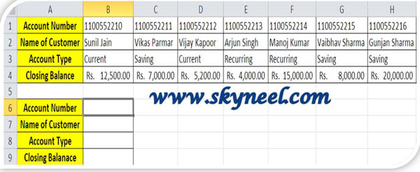
Step 1: Prepare the following given database in excel sheet.
Note: You can also copy the range of cell A2:D14 from Sheet 1 and take cursor on another sheet or workbook like A1 of Sheet 2 > Click Home tab > Click Paste Special > Turn “ON” Transpose option in Paste Special dialog box > Click OK button.
Must Read: Vlookup merge data from one sheet to another Excel worksheet
Step 2: To view the customer name take cursor on cell B8 and type the following given formula: =HLOOKUP($B$7,$B$1:$N$4,2,0) when you press enter, excel displays an error message #N/A. Because you don’t fill account number of the customer in the cell B7.
Step 3: To view the customer account type take cursor on cell B9 and type the following given formula like this, change the value of row_index_num: =HLOOKUP($B$7,$B$1:$N$4,3,0)
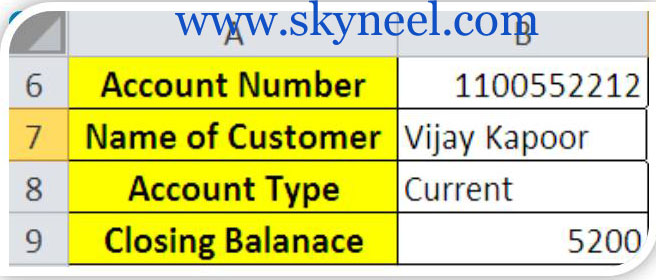
Step 4: To view the closing balance of customer take cursor on cell B10 and type the following given formula like this, change the value of row_index_num:=HLOOKUP($B$7,$B$1:$N$4,4,0). After applying the formula it shows following result.
Note: After applying all formulas, insert account number of any customer in cell B7, excel automatically displays values of all cells.
I hope you like this Vlookup and Hlookup Functions guide, please give your important suggestions in the comment box and also share your knowledge with your friends, colleague, family members and others. Thanks.


💬 Loading comments...