Hi, everyone today we discuss very important topic which you face during doing job in your company or facing the interview session. How to compare values in different Excel sheet and also want to make formatting of those values which are not matched as per the given condition? After reading this important article you will be able to easily VLOOKUP Compare values in another Excel worksheet data with the help of VLookup Function in MS Excel.
VLOOKUP Compare values in another Excel worksheet:
The answer to this query is only one you can easily use most popular “Vlookup” function which exist in the lookup and reference category of Microsoft Excel and you can also use the Conditional Formatting feature to fill background color and draw borders on those cell values which are not matched as per given condition. So have a look and take few easy steps to easily overcome this kind of problem.
Must Read: MS Excel : Vlookup Function with a Spreadsheet
Syntax of Vlookup:
The Microsoft Excel VLOOKUP function search a value in the extreme left column of the table_array and provide the value in the same row which is based on the index_number.
=VLOOKUP(lookup_value,table_array, col_index_num, [range])
Note: Before using the Vlookup function, first you need to arrange first column of table or array in the ascending order, otherwise VLOOKUP function is not able to provide the accurate result.
Lookup_value: The value to be searched in the extreme first column of the table array.
Table_array: Two or more columns of data. Give cell reference of a range / range name.
Col_index_num: The column index_number in the table from which the searched value must be returned. If col_index_num of returns 1 the value in the first column in table_array.If col_index_num is: Less than 1, this function returns an error value the #VALUE!. If it is a greater than the number of columns in table_array, this function returns error value #REF!.
Range_lookup: It is an options part of this function.
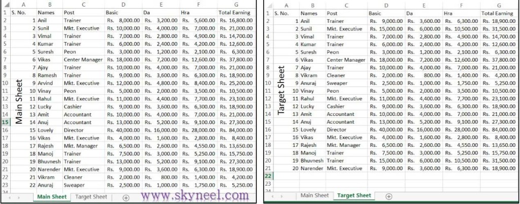
For example, you have a two different sheet which has the same kind of data, but some data are changed or missing in second sheet, now if you want to compare both sheet data on the basis of the basic salary column then you have to take few given steps.
There is same column heading of both sheet data’s are given below:
A1= “S. No” B1= “Names”, C1= “Post”, D1= “Basic”, E1= “Da”, F1= “Hra”, G1= “Total Earning”.
Step 1: Fill the required data in main sheet and target sheet as per the requirement of your company. But both sheets have few changes, in main sheet you fill only 22 records as per given below and in target sheet you fill only 20 records and also make some modification in target sheet data.
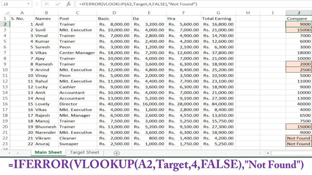
Step 2: Select the data of “Target Sheet” A2: G21 and given the name “Target” from the Name box window. Now, if you want to find the comparison between both sheets, then first you have to type the “Compare Result” on cell J1 in the “Main Sheet”, and type the following given formula in cell J2 = VLOOKUP(A2,Target,4,FALSE).
Step 3: Now, drag the formula with the help of a mouse button up to cell J22, or select the range of cell J2:J23 then press the Ctrl+D shortcut key. Note: Some cells display the result #N/A, if you want to remove this error, then you have to update your vlookup formula by using the “IFERROR” function.
Must Read: Use Data Validation, Naming the range and VLookup Function
Step 4: Again open the formula of cell J2 and update the existing formula from this formula. =IFERROR(VLOOKUP(A2,Target,4,FALSE),”Not Found”). Now drag the range of cell up to J23. Now, you are watching it shows “Not Found” at the place of error message #N/A.
Step 5: If you want to make conditional formatting on the compare result data, then first you have to select the range of cells J2:J23 and click on the Home >>> Conditional Formatting >>> Then after click on the New Rule option >>> Now Select “Use a formula to determine which cells to format” option and type the following formula =J2<>D2 in “New Formatting Rule” dialog box.
If you want to make background color and draw borders on those cell data which are not matched then click on the Format button and fill and required color from the Fill tab and also select any required border format from the Border tab >>> Click OK button >>> Again click OK button.
I hope you like this guide from which you will be able to easily VLOOKUP Compare values in another Excel worksheet without any extra efforts. If feel any problem in this guide then please use comment box. Thanks to all.


💬 Loading comments...