Hi, today we are talking on The Excel FV – Future Value Function allows you to return the future value of an investment which is based on a periodic, constant interest rate, constant payments. Future value is an important and popular function which is located in the financial category. You can check this function from Formula tab then Financial functions library.
For Example:
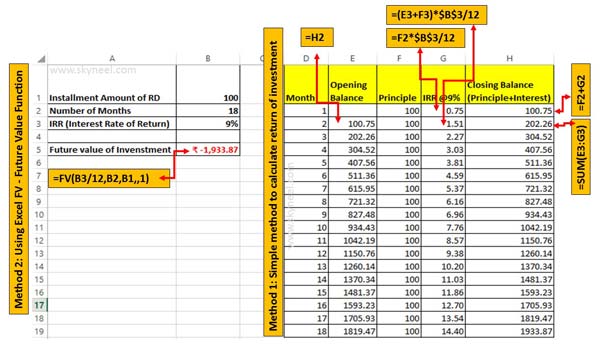
In the given spreadsheet, the Excel FV function is used to calculate the future value of an investment of $100 per month for the period of 18 months. The present value is 0, the interest rate is 9% per year. Now you want to know how much amount you will get after the 18 months as per the investment.
Must Read: How to Age calculation From Date of Birth – MS EXCEL
All we know we have to pay monthly instalment and the annual interest rate is 9%. Now you have to change annual interest rate 9% into monthly basis (=9%/12) during using the formula. Before start the process how to use Excel FV future value function you must have to know few important things.
How to use Excel FV – Future Value Function
To get the future value of an investment you must have to use Excel FV function in active worksheet.
Syntax of Excel FV function: FV(rate,nper,pmt,[pv],[type])
Important Arguments of FV function:
Rate: The required interest rate per period.
Nper: The required total number of payment periods in an annuity.
Pmt: The payment made each period; it cannot change over the life of the annuity. It is an required argument.
Pv: It’s an option argument.The present value, or the lump-sum amount that a series of future payments is worth right now.
Type: It is another an optional argument. The number 0 or 1 and indicates when payments are due. If type is omitted, it is assumed to be 0. 0 means at the end of the period while 1 at the beginning of the period.

Method 1: Simple method to calculate return of investment
Step 1: Create the following structure to get the future value of investment.
Step 2: Type the following given formula in cell G2 =F2*$B$3/12 to get the monthly interest amount. Just like this calculate closing balance (Principle+Interest) in cell H2 =F2+G2 and press enter. The closing balance will be the opening balance for next month.
Must Read: How to Search Duplicate Values with VLookup function
Step 3: Set the following formula to get the cumulative interest amount in cell G3 =(E3+F3)*$B$3/12. Now get the closing balance till second instalment using given formula in cell H3 =SUM(E3:G3) and press enter to get the result. Copy the E3, G3 and H3 formula for rest of the cells.
Step 4: Finally you can check at the end of the 18 months you will get final return of investment against the monthly recurring deposit.
Method 2: Using Excel FV – Future Value Function to calculate return of investment
There is another way which you have to use to calculate return of investment using the FV means Future Value function in Excel. To get the future value against the investment for specific period, interest rate you have to take following given steps.
Step 1: Create the following structure to get the future value of investment.
Step 2: Apply the following given function in cell B5 =FV(B3/12,B2,B1,,1). Now press enter to get the future value of an investment.
After using given both methods you can check you will get same result against the investment. If you have any suggestion regarding this article then please write us in the comment box. Thanks to all.
💬 Loading comments...