Hi Guys we know very well about the importance of VLookup and Match functions in MS Excel. There are variety of built-in functions in MS Excel. So, today we have to discuss how to use VLookup multiple criteria using Match function in MS Excel.
Most of the time we have to apply multiple criteria to search any specific value but VLookup does not support multiple conditions.
If we have to apply multiple criteria to search any value in that situation you have to combine VLookup with Match function to get the result. VLookup is an important function which is used to find and specific value which match the given criteria. While Match function return the relative position of any item in any table or an array that match the specified value in a specific order.
VLookup multiple criteria using Match function
If you need to search multiple criteria and get the exact result then you have to used more than one function. This article helps you how to use VLookup multiple criteria using Match function.
If you have a large worksheet or database in which there are multiple records which have same information in few columns. In that situation you must have to apply VLookup function to search any specific value, you will get the first one as the result.
Sometime you need to apply more than one criteria to match any specific data but you can’t get the exact result. Now VLookup allows you to use multiple criteria using Match function to get the exact result. First we have to discuss about the VLookup and Match function, have a look:
Definition and Syntax of VLookup Function:
VLookup is a great function which is found in the “Lookup and Reference” categories in MS Excel. VLookup function is used to lookup a value in the left most column of a table. After that this function return a value in the same row from a column you specify.
The VLookup function searches a value in the extreme left column of the table_array and provides the value in the same row which is based on the index number.
Must Read: How to use VLookup function with multiple criteria
= VLookup (lookup_value, table_array, col_index_num, [range])
Note: Before using the VLookup function, first you need to arrange first column of a table or array in the ascending order, otherwise VLookup function is not able to provide the accurate result.
Lookup_value: The value to be searched in the extreme first column of the table array.
Table_array: Two or more columns of data. Give cell reference of a range / range name.
Col_index_num: It is the column number in the active table from which the searched value must be returned.
If col_index_num of returns 1 the value in the first column in table_array.
If col_index_num is: Less than 1, this function returns an error value the #VALUE!.
If it is a greater than the number of columns in table_array, this function returns error value #REF!.
Range_lookup: It is an options part of this function. There are two options available in this part.
TRUE- Appropriate Match. This option work properly when the first column of your table is sorted in the ascending order.
False: Exact Match: VLookup by default check only on exact match method.
Definition and Syntax of Match Function:
Match function is used to search specific value in the active worksheet. Now this function return the exact position of the value in the given range.
MATCH(lookup_value, lookup_array, [match_type])
lookup_value: Lookup values is the value which is search in the table array.
lookup_array: It is the range of cells in which you have to search lookup_value.
match_type: It’s an optional. The default value is 1. The number -1, 0, or 1.
1: Used to find the largest value that is less than or equal to lookup_value.
2: Used to find the first value that is exactly same to lookup_value.
-1: Used to find the smallest value that is greater than or equal to lookup_value.
Must Read: Remove spaces with Data Validation in MS Excel
Step how to apply VLookup multiple criteria using Match function
Sometime you need to search multiple criteria in the active worksheet. In that situation you have to combine VLookup with Match function to get the result.
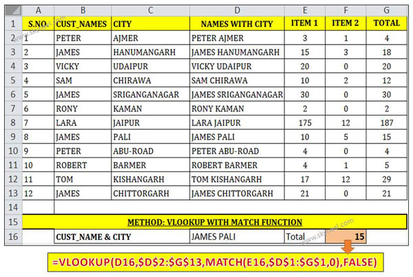
Step 1: Create the following table to start the searching process.
Step 2: Take the cursor on cell F16 and type the following formula:
=VLOOKUP(D16,$D$2:$G$13,MATCH(E16,$D$1:$G$1,0),FALSE)
Step 3: After typing the formula press enter key to get the result. Now, you will get the final result 15. This function search “James” who lives in the “Pali” city.
I hope you like this article, after reading it you will be able to easily apply VLookup multiple criteria using Match function. Both function helps you get the exact result as per your need. Give your important suggestion regarding this article in the comment box. Thanks to all.

💬 Loading comments...