Hi, friends today we discuss about the most important and popular rank function in MS Excel. This is very important statistical function which is used to verify or test the rank of any number from given range of cells. This functions show rank of any number after comparing with other numbers in the range of cells or active table or an entire worksheet. RANK function, assigns a rank based on the size of a number compared to the other figures in the list.
🔥 Trending: How to download Voter ID Card in Smartphone
✅ Must Read: What is E-PASSPORT, Its FEATURES and How to Apply E-Passport
The syntax for the RANK function is:
= RANK (Number, Ref, Order)
Number / figures – Cell reference of the given figure to be ranked.
Ref – Range of cells to use in the position the figures.
Order – Either given numeric is ranked in the Increasing or Decreasing order.
Type “0” (nil value) which is used for provide position in decreasing order (largest to smallest).
Type “1” (one) to provide position in the increasing order (smallest to largest).
Example:
How to use Excel’s RANK Function
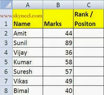
1. Prepare following sheet given below in range A1:C8.
👉 Don't miss: What is the Clear signs to know your phone was hacked
🔥 Trending: DCOUNT Database Function of MS Excel
2. Click to the C2 cell reference – the place where you want to view the result.
3. Drag select cells C4 to C13 in the worksheet which is used to feed the range in the box.
4. In [order] in the dialog box, type 0 (zero) to get the position of the number in descending order.
5. Click on cell B2 to view the number which you want to ranked (85).
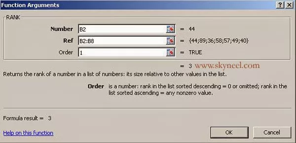
6. Click on “Ref” line and drag select cells B2 to B8 in the worksheet to enter the range into the given dialogue box.
7. Click on “Order” line in and type one on this line to rank the number in ascending order >>> Click OK button. The number 3 displays in the cell C2 since the number 44 is the third largest number.
8 After clicking on the cell C2, formula bar display the function = RANK (B2, B2:B8,1). You are able to to do any kind of modification in your formula from formula bar.
9. Now if you want to copy this formula on rest of the cell then first open this formula by double clicking on cell C2 or you can also select cell C2 then press F2 function key.
10. Select the range B2:B8 then press F4 function key to change the cell reference type in absolute format like $B$2:$B$8 to fix this range then drag this formula on rest of the cells.
11. It automatically copy all formula on all cells and displays the result as per given below.
I hope you like this Excel RANK Function guide. Give your important suggestion in the comment box and also share this article with your friends to show your knowledge in excel. Thanks.


💬 Loading comments...