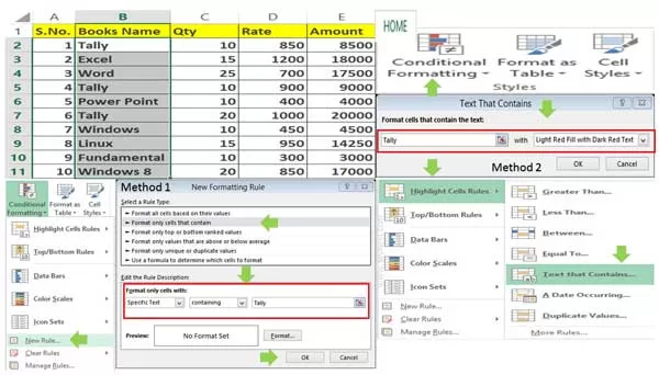
During working on large worksheet you must need to highlight few cells on particular text and this could be done with Conditional formatting. In this article we have to discuss how could you easily to highlighted cells which have specific text using Conditional formatting feature in Excel.
Also see:
- How to download Voter ID Card in Smartphone
- What is E-PASSPORT, Its FEATURES and How to Apply E-Passport
Conditional Formatting is an important tool of Microsoft Excel. Conditional formatting allows you to quickly apply the formatting on particulars cell or range of cell contents. There are lot of options which you have to use you have to use when you want to apply conditional formatting on selected range of cells. You can apply conditional formatting on particular text, numbers, date or apply any function on selected range of cells. You can also edit or remove the apply conditional formatting on selected range of cells or entire worksheet.
Must Read: How to find duplicates using conditional formatting in Excel
Highlight Cells Containing Specific Text with Conditional Formatting
During working on the spreadsheet you have to quickly highlight the important information to take your attention. There is few built in formatting rules which you have to apply as per your need. You can also create your own rules with the help of function to apply conditional formatting on active worksheet.
For eg: If you want to highlight all those cells in which you have only those books name which match with the “Tally”. In that situation you have to use Conditional formatting feature on active worksheet.
Must Read:
- How to clean Google Play Store apps and search history
- How to get more free storage space in Android Phone

First Method:
Step 1: Select the range of cells in which you want to highlight cells containing specific text with Conditional formatting.
Step 2: Click on the Home > Conditional Formatting > New Rule… option. In the Rule Type box choose “Format only cells that contain” option.
Step 3: Choose Specific Text option and type the text name which you want to highlight with the help of conditional formatting.
Step 4: Click on the Format button and fill the required color, border, font as per your need and click on the OK button. Again click on the OK button to highlight cells containing specific text with conditional formatting in active worksheet.
Must Read: Conditional Formatting : Highlighted Weekends in Excel
Method 2:
This is quick way which allows you to apply conditional formatting on particular text on the selected range of cells. You have to take few given simple steps to do this job, have a look.
Step 1: First you have to select the range of cells.
Step 2: Home > Conditional Formatting > Click on the Highlight Cells Rules > Click on the Text that Contains… option.
Must Read: Conditional Formatting – How to generate chess board on excel
Step 3: Type the specific text which you want to highlight and set the required formatting as per your requirement. Now, click on the OK button to highlight cells containing specific text with Conditional formatting.
We just share want to share our knowledge with all those guys who relay want to do few important things. If you have any query or suggestion regarding this guide then please write us in the comment box. Thanks to all.
💬 Loading comments...