Match function in Excel allows you to search for a value in an array and return the relative position of the item in specific order. Sometime you need to apply more than one criteria in that case you can use Match function in Excel. Excel Match function is an important function which is located in Lookup and Reference category.
Match function in Excel allows you to apply multiple criteria and find the relative position of the given item. Excel provide several ways like VLookup to search more than one criteria with VLookup function. You can also use Match and Index function to search the specific value relative position.
Must Read: MS Excel DMIN Database Function
How to apply multiple criteria using match function in Excel
If you want to know how to apply multiple criteria using Match function, then first you must know about this function.
Syntax of Match Function in Excel
MATCH(lookup_value, lookup_array, [match_type])
lookup_value: The value that you want to match in lookup_array. It can be a number, text, logical value or a cell reference.
lookup_array: It is the range of cells being searched.
match_type: It’s an optional value. You can put the number -1, 0, or 1 in match type. The default value for this argument is 1.
1: Match function finds the largest value that is less than or equal to lookup_value.
0: Match finds the first value that is exactly equal to lookup_value.
-1: Match finds the smallest value that is greater than or equal to lookup_value.
Must Read: How to use Advance Backward VLookup in Reverse Order in Excel
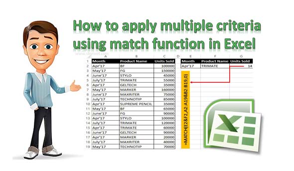
For eg: If you have a worksheet data in which you have Month Name, Product Name and Number of Units sold.
Steps to apply more than one criteria using match function in Excel
You have to take few given simple steps which allows you to use Match function with more than one criteria.

Step 1: Create the following given worksheet to start the process of multiple criteria using the match function.
Step 2: Now you want to search number of units sold which match the given month and product name. Fill the month name in E2 and Product name in F2. Now apply the following given function in cell G2 to get the result using Match function.
=MATCH(E2&F2,A2:A19&B2:B19,0) Now press Ctrl+Shift+Enter key to get the result.
I hope after reading this guide you can easily understand how to apply multiple criteria using match function. If you have any suggestion regarding this guide then write us your suggestion in the comment box. Thanks to all.
💬 Loading comments...