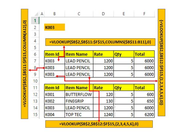
With the combination of Excel VLOOKUP function with the Column, Column and array function you can easily create a lookup formula which allows you to quickly lookup multiple fields of data with Excel VLookup function. Excel VLookup function with array or column function easily return multiple values from a single row of a database or array of table.
In this guide we explain different methods which helps you to quickly get the result of multiple fields value with Excel VLookup function.
The VLookup function requires to use the Columns or Column functions to be nested inside of VLOOKUP. Nesting with in a function involves entering the second function as one of the arguments for the first function. In this guide, you can use array number, column or columns function as the column index number.
Step to Lookup Multiple Fields of Data with Excel VLOOKUP
Step 1: First you must have to enter few data into an Excel worksheet. You can take help of given image in which data is entered in specific format. You can change the order or data as per your need.

Step 2: In this guide we explain three different methods which helps you to quickly return multiple values with Excel VLOOKUP function.
Method 1: Using Columns function:
In given method you must have to use Columns function to quickly lookup multiple fields of data with Excel VLOOKUP function. In this method you have to type the given function in Cell B7 =VLOOKUP($B$2,$B$11:$F$15,COLUMNS($B$11:B11),0) and press enter.
Now, drag the given function for rest of the cells to get the result.
Method 2: Using Column function:
You can also use Column function to get the result of multiple fields of data with Excel VLOOKUP function. In the given method you have to given function in Cell B8 =VLOOKUP($B$2,$B$11:$F$15,COLUMN (A12),0). Drag the given function for all the cells to view the result.
Method 3: Using Array:
In third method you can use array with combination of VLOOKUP function to get the result. To get the result as per the given method type of given function in Cell B9 =VLOOKUP($B$2,$B$12:$F$15,{1,2,3,4,5,6},0). For rest of the cells you have to do little bit correction in array you the function.
Cell C9 =VLOOKUP($B$2,$B$12:$F$15,{2,3,4,5,6},0).
Cell D9 =VLOOKUP($B$2,$B$12:$F$15,{3,4,5,6},0)
💬 Loading comments...