Match function found in Lookup and reference category in Excel. This function allows you to quickly locate for a specified item in range of cells, and then returns the relative position of that item in the range. Match Excel Function is used to returns the relative position of an item in the given array or range of cells that match a specific value in specific order. You can easily use this function to get the result either in vertical or horizontal lookup array.
Must Read: Excel Index Match Min to Lookup minimum Value
In this tutorial we have to explain how to use Match function in Excel. You can use this function with Index function at the place of VLookup function. If you need to use advance lookup then you have to use Index Match or VLookup function. In Microsoft Excel there are lot of text function which allows you to find a particular text or string. This function designed to get the relative position of an item in given range of array.
MATCH (lookup value, lookup array, [match_type] )
lookup_value: The value that you want to match in lookup_array. The lookup_value argument can be any number, text, logical value or a cell reference to a number, text, or logical value.
lookup_array: It is range of cells being searched.
match_type: It is an optional. The number -1, 0, or 1. The match_type argument specifies how Excel matches lookup_value with values in lookup_array. By default value for this argument is 1.
How to use the Match function in Excel
If you want to use the this function in Excel then you have to take few given simple steps have a look.
Must Read: Excel VLookup Find First, 2nd Or Nth Match Value in Excel?
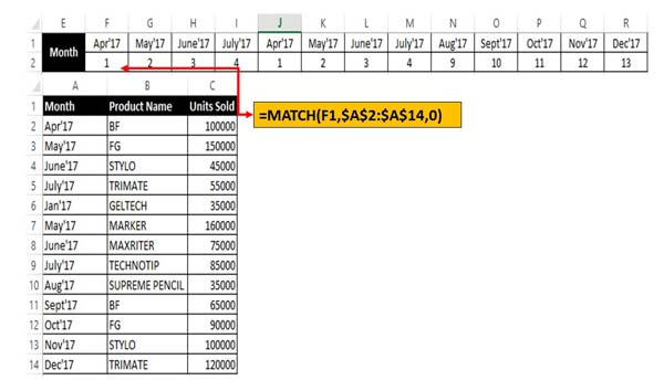
For eg: If you have list of month, product name and units sold. Now you want to know relative position of particular month then you have to use match function to get the result.

Step 1: Prepare the following sheet to get the relative position of month name.
Step 2: Type the given function in cell F2 =MATCH(F1,$A$2:$A$14,0).
Step 3: Drag the match function of cell F2 to R2 to get the relative position of particular month in the active table array. You must have to note before drag the function you must have to change the lookup array in absolute reference.
You must have to remember few important things that Match Excel function is not case sensitive. If match function not able to found the lookup value it returns #N/A error value.
💬 Loading comments...