Solver is an another important utility of Microsoft Excel. With the help of solver you can easily find an optional value which is also called objective cell that satisfies all constraints and maximize or minimize the objective cell value. In this article we have to discuss how to use solver command in Microsoft Excel.
Also see:
- How to download Voter ID Card in Smartphone
- What is E-PASSPORT, Its FEATURES and How to Apply E-Passport
Solver is an important utility of What-If-Analysis. Solver command works with group of cells. You can also know as a decision variables. With the help of solver command you can easily adjust the values in the decision variable cells. You can easily adjust the value in decision variable cell which satisfy the constraint cells limits. After that solver command produce the result which you want for the objective cell. If you want to optimizing values in the active worksheet which meet the object
Must Read: Conditional Formatting – How to generate chess board on excel
For eg. If you have seven items in the list and total of all these items is 70000. Now, you want to increase the final amount up up to 84000 and equally divide all extra amount between all the items. In that situation you can use solver command in the Microsoft Excel. Solver and Goal Seek is an important part of What-If-Analysis in Microsoft Excel.
How to active solver command in MS Excel 2010
Must Read:
- How to unlock bootloader BQ Aquaris M5 Smartphone
- 2 Ways to Fill blank cells with 0 or any specific value in Excel

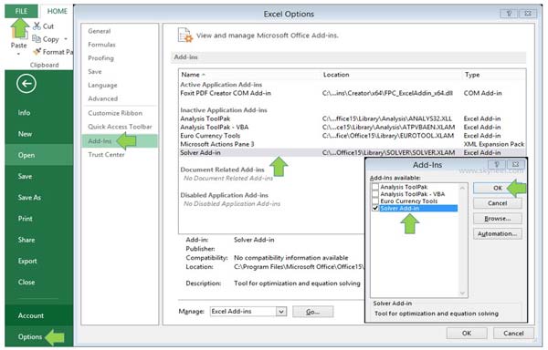
Step 1: Click on the “File” menu > Click on the “Option” command.
Step 2: Click on the “Add-Ins” category in the Excel options dialogue box.
Step 3: Select “Solver Add-in” in the right pane. Click on the drop down arrow of Manage box and choose “Excel Add-ins” option. Click on the “Go…” button.
Step 4: Turn on “Solver Add-in” in the Add-Ins dialogue box and click on the OK button. Now, solver command is available in the Data tab.
How to use Solver command in Microsoft Excel
If you want to get required final result and equally divide difference amount between the all items equally than you can use solver command in Excel.

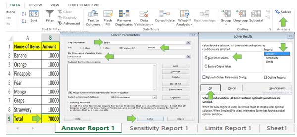
Step 1: Create given table in the Microsoft Excel.
Step 2: Select the cell B9 and calculate the total of all items by typing the given formula =SUM(B2:B8).
Step 3: Click on the “Data” tab > Click on the “Solver” command.
Step 4: Fill $B$9 absolute cell address in the Set Objective box. Select “Value Of” option in the “To” and fill the required resulted value in the box.
Must Read: How to freeze or lock rows and columns in Excel at the same time
Step 5: Click on the “Solve” button. Turn on “Keep Solver Solution” option and select any required reports in the “Reports” section. Now, click on the OK button to get the final result.
As per the given example the total of all seven items is 70000. When you set 84000 final value in the solver parameter box you can see the different amount 14000 is equally divided in the seven items.
As per the requirement there are different situations in which you can use solver command in MS Excel. I hope after reading this guide and example you can easily understand how to use solver command in Excel. If you have any query regarding this article please write us in the comment box. Thanks to all.
💬 Loading comments...