All we know very well importance of MS Excel. What If Analysis is an important part of Microsoft Excel. Today we have to discuss an easy way to create What IF Analysis data table in MS Excel.
👉 Don't miss: How to download Voter ID Card in Smartphone
🔥 Trending: What is E-PASSPORT, Its FEATURES and How to Apply E-Passport
MS Excel is an electronic spreadsheet software which is used to create, edit different kind of data, prepare different types of charts, solve complex calculations with the help of functions and many more.
What If Analysis:
What If Analysis is an important part of MS Excel. With the help of What If Analysis you will be able to easily modify the cell values and view how these modifications are taking affect on the result of formula on the active worksheet. For example, varying the interest rate and term that is used in an amortization table to determine the amount of the payments.
For e.g.: If you want to take loan from any bank or finance company. But you want to compare instalment amount which is based on different interest rate and different period. Now, you want to know if period and interest amount is changed then what effect is done of instalment amount, in that situation you have to create What IF Analysis data table in MS Excel.
Must Read: How to quickly remove all blank cells in MS Excel
How to create What IF Analysis Data Table in MS Excel:
Data table is an important part of What if analysis. With the help of data table you will be able to easily change one or more than one variable values and watch the result on active worksheet. This article provide you an easy way to create What IF Analysis data table in MS Excel.
One Input-Data table:
One input data table is an important part of What if analysis in MS Excel. With the help of one input data table you will be able to modify any single variable value in your active worksheet. After that view how to change the values for that variable affect the values of calculated by one or more formulas in the active worksheet.
💡 You might like: How to recover lost contact list from Gmail on Android phone
👉 Don't miss: How To Download Facebook Videos in HD Quality
Steps to create One Input data table:
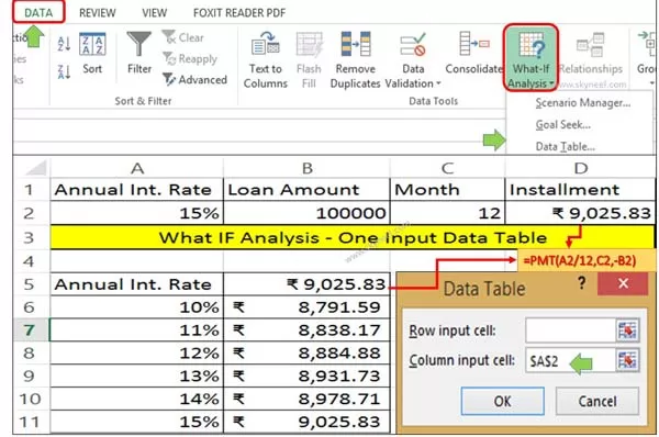
Step 1: You have to create following given table in active worksheet.
Step 2: Take cursor on cell D2 and type the following given formula to calculation per month instalment. =PMT(A2/12,C2,-B2)
Step 3: Again type same formula in the cell B5 =PMT(A2/12,C2,-B2). Select the range A5:B12 and click on the Data tab.
Step 4: Click on the What If Analysis option and select Data table option. It will display data table dialogue box. Now, type $A$2 in the column input cell box and click on the OK button. Now, you will get the instalment amount till selected range of columns.
Two Input Data table:
Two input data table in another important part of What if analysis in MS Excel. With the help of two input table table you will be able to modify two variable values in your active worksheet. After that view how to change the values for that variable affect the values of calculated by on or more formulas in the active worksheet.
Must Read: VLookup function with two lookup values in Microsoft Excel
Steps to create Two Input data table:
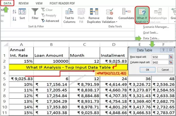
Step 1: You have to create following given table in active worksheet.
Step 2: Take cursor on cell D2 and type the following given formula to calculation per month instalment. =PMT(A2/12,C2,-B2)
Step 3: Again type following formula =PMT(A2/12,C2,-B2) in cell A5. Select the range A5:F12 and click on the What If Analysis option and select the Data table from Data tab. Type $C$2 in the Row Input box and $A$2 in Column Input box and click on the OK button. Now, Excel automatically calculate the result in the range of cells B6:F12.
Must Read: How to hide spelling and grammatical errors from MS Word
I hope you like this article after that you will get an easy way to create What IF Analysis data table in MS Excel. If you have any suggestion regarding this article then write us in the comment box. Thanks to all.


💬 Loading comments...