Today, we learn how to use the Excel SUMIF function with an example. This function is used to add all the numeric value of cells as per specified by given condition. SUMIF function allows you to add all numeric values within given range (more than one contiguous cells) of cells.
This function is very useful when sometimes you needs to added up the cells that meet certified norms. We already discuss different ways to use SUM function in MS Excel in another post. Syntax of SUMIF function=SUMIF(range, criteria, [sum_range]) range is the range of cells you want to added up. It is required for the function to work.criteria is the criteria which must be met for a cell to be included in the total. It is also required.
Must Read: How to Restrictions on Columns by Data Validation in Excel
sum_range is the range of cells that will be added up. It is optional; if you leave it out, Excel will check the criteria against the sum_range. In the two examples above, the first example doesn’t need you to provide a sum_range, while the second example does. Now, have look an easiest way to use this function, we have to take an example in excel sheet- If you want to calculate total amount of those fruits which name is “Apple”, in that case you have to use SUMIF function very easily.
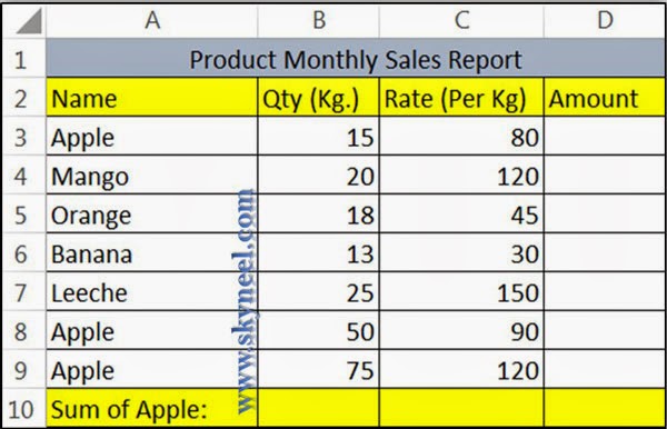
Step 1: Prepare following sheet i.e. Name, Qty, Rate and Amount & feed some records given below.
Step 2: Place cursor of Cell D3 and type following formula to get amount by multiplying Qty * Rate =B3*C3 and copy this formula up to cell D9 by dragging mouse button.
Must Read: Conditional Formatting : Highlighted Weekends in Excel
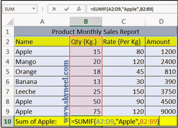
Step 3: If you want to get total Qty, Rate and Amount only for “Apple” Product then type following formula in given cells:
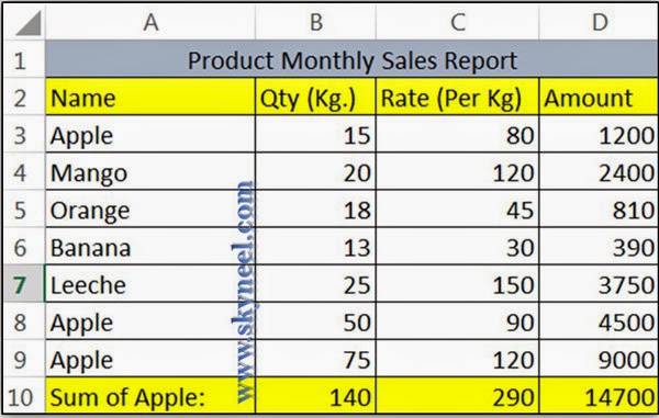
Cell B10 =SUMIF(A2:D9,”Apple”,B2:B9) Result = 140
Cell C10 =SUMIF(A2:D9,”Apple”,C2:C9) Result = 290
Cell D10 =SUMIF(A2:D9,”Apple”,D2:D9 Result = 14700
Step 4: After applying all formulas you will get this resulted sheet:
I hope you like this post. Give your important suggestion in the comment box and also share this article with your friends, office staff members and many more to show your knowledge in excel. Thanks.


💬 Loading comments...