Sometime we need to apply triple VLookup in active worksheet and want to get the result which fulfil all given three criteria. In that situation you must have to use Index Match function at the place of applying VLookup function in active worksheet. In this article we have to discussion how could you easily apply triple VLookup with Index Match function in active worksheet.
Must Read: How to use Double VLookup in Excel
If you have a table in which you have more than two criteria and now you want to get the specific column value result which match all the given condition. Most of the Excel users make lot of complex formula to get the result in that situation. Now you have to use Index and match function at the place of triple VLookup in active worksheet to get the result.
Triple VLookup with Index Match function in Excel
To lookup multiple column values you have to use INDEX MATCH function in Excel. Before we start this function you must have to know about the Index and Match function in Excel.
Index Function in Excel
Index function return a value or the reference number to a value from given range of cells or table array.
👉 Don't miss: How to download Voter ID Card in Smartphone
🔥 Trending: What is E-PASSPORT, Its FEATURES and How to Apply E-Passport
INDEX(array, row_num, [column_num])
Array : It is a range of cells or an array constant.
👉 Don't miss: How to unlock bootloader LG Devices (All Models)
🔥 Trending: How to send images without spoiling quality on WhatsApp
Row_num : Selects the row number in an array from which to return a value. If Row_num is omitted, Column_num is required.
Column_num : It is an optional. Selects the column number in an array from which to return a value. If Column_num is omitted, Row_num is required.
Match Function in Excel
Match function used to returns the relative position of an item in the given array or range of cells. This function match the specific value in specific order.
MATCH (lookup value, lookup array, [match_type] )
lookup_value: The value that you want to match in lookup_array. The lookup_value argument can be any number, text, logical value or a cell reference to a number, text, or logical value.
lookup_array: It is range of cells being searched.
match_type: It is an optional. The number -1, 0, or 1. The match_type argument specifies how Excel matches lookup_value with values in lookup_array. By default value for this argument is 1.
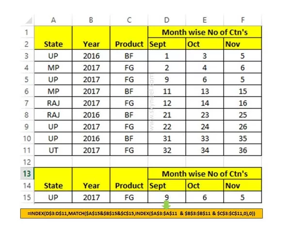
For e.g.: If you want to match State, Year and Product criteria and want to get the month wise number of ctn’s as a result. In that situation you have to use given Index and Match function in Excel for triple VLookup.

Step 1: Prepare the following table structure to know how to use triple VLookup with Index Match function in Excel.
Must Read: Search Index Match Lookup multiple columns Value with Index Match Function
Step 2: Apple given function in Cell D15 to get Sept month number of Ctns
=INDEX(D$3:D$11,MATCH($A$15&$B$15&$C$15,INDEX($A$3:$A$11 & $B$3:$B$11 & $C$3:$C$11,0),0))
Step 3: Now drag or copy the given function for get the number of ctns for the month of Oct and Nov which fulfil the given triple conditions.
I hope after reading this guide you can understand how to apply triple VLookup with Index Match function in Excel. If you have any suggestion regarding this guide then please let me know via comment box.
💬 Loading comments...