Just like VLookup function, Match and Index function also used for lookup purpose in Microsoft Excel. Index Match function in Excel works right to left, while VLookup works left to right. In this guide we have to discuss how to use Index Match function in Excel.
Also see:
- How to download Voter ID Card in Smartphone
- What is E-PASSPORT, Its FEATURES and How to Apply E-Passport
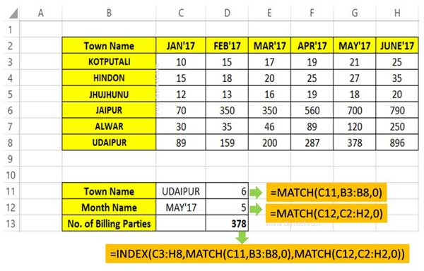
Index Match function in Excel allows you to search the specific value from right to left and also reduce the load time. For eg. If you have an worksheet in which you want to search the number of billing parties town wise and month wise. In that situation you have to use Index Match function in Excel to get the exact result.
How to use Index Match function in Excel
Excel is an important utility electronic spreadsheet software. There are lot of variety of function which is used to solve complex calculations. VLookup is one of the most important functions which are found in “Lookup and Reference” category of Microsoft Excel. It is used to searches for a value in the extreme left column of the table_array and provides the value in the same row which is based on the index number.
Must Read: Advanced VLookup trick with Data Validation in Excel
Index Function in Excel
Index function return a value or the reference number to a value from given range of cells or table array.
Must Read:
- How to Watch YouTube Videos in Fast or Slow Motion
- Aadhaar Card getting lost ? Order Reprint Aadhaar Card
INDEX(array, row_num, [column_num])
Array : It is a range of cells or an array constant.
Row_num : Selects the row number in an array from which to return a value. If Row_num is omitted, Column_num is required.
Column_num : It is an optional. Selects the column number in an array from which to return a value. If Column_num is omitted, Row_num is required.
Match Function in Excel
This function is used to returns the relative position of an item in the given array or range of cells that match a specific value in specific order.
MATCH (lookup value, lookup array, [match_type] )
lookup_value: The value that you want to match in lookup_array. The lookup_value argument can be any number, text, logical value or a cell reference to a number, text, or logical value.
lookup_array: It is range of cells being searched.
match_type: It is an optional. The number -1, 0, or 1. The match_type argument specifies how Excel matches lookup_value with values in lookup_array. By default value for this argument is 1.
Must Read: How to use Flash Fill or Auto Fill command in Excel
Step how to use Index Match function in Excel
If you want to use use both Index Match function in Excel to search the value, then you have to take given steps.

Step 1: Create the given worksheet in Excel.
Step 2: Prepare the drop down town name list in cell C11 with the help of Data validation command in Excel. You can also create the month name list in cell C12 with the help of Data validation in Excel.
Step 3: Use the given match function to find the relative position of town name in Cell D11 =MATCH(C11,B3:B8,0). You can find out the relative position of month name with the help of given function in cell D12 =MATCH(C12,C2:H2,0).
Step 4: To find out number of billing parties which match the specific town and month relative position, you have to use Index Match function in Excel. Type the following function in the cell D13 =INDEX(C3:H8,MATCH(C11,B3:B8,0),MATCH(C12,C2:H2,0)).
Must Read: How to use Solver command in Microsoft Excel
I hope this guide is useful for all those guys who want to use Index Match function in Excel in single cell. If you have any suggestion or query regarding this guide then please write us in the comment box. Thanks to all.
💬 Loading comments...