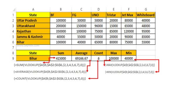
In this guide, you will find a very helpful advanced VLookup formula which demonstrate how to use VLookup to Get Sum, Average, Count, Maximum and Minimum value from Multiple Columns. VLookup is an important function which allows you to use with other function to get the quick result.
Also see:
- How to download Voter ID Card in Smartphone
- What is E-PASSPORT, Its FEATURES and How to Apply E-Passport
Must Read: How to use Advance Backward VLookup in Reverse Order in Excel
Sometime during working on Excel sheet you need to use a VLookup to get values for Multiple columns. Most of person try to get the result which match the condition in normal process then your most of time consumed. If you don’t have enough time then you must have to use VLookup function in Excel to lookup the value. If you need to calculate different result which match the condition in that situation you must have to know read this guide. You can use VLookup function with Sum, Average, Count, Max and Min functions to get the result which match the condition.
For eg: If you have different products sales amount of different state. Now, you want to calculate the Sum, Average, Count, Max & Minimum value which match the State. In that situation you have to use VLookup with these functions to get the quick result.
How to use VLookup to Get Sum, Average, Count, Maximum and Minimum value from Multiple Columns

Must Read:
To get the sum of all the products which match the state type the function in Cell B9.=SUM(VLOOKUP($A$9,$A$2:$G$6,{2,3,4,5,6,7},0)). After typing the function press Ctrl+Shift+Enter at the place of Enter key to get the result.
To get the average of all the products which match the given state type the function in Cell C9.=AVERAGE(VLOOKUP($A$9,$A$2:$G$6,{2,3,4,5,6,7},0)). After typing the function press Ctrl+Shift+Enter to get the average of all products which match the state.
Must Read: Excel VLookup Find First, 2nd Or Nth Match Value in Excel?
To get the count of all the products which match the given state type the function in Cell D9.=COUNT(VLOOKUP($A$9,$A$2:$G$6,{2,3,4,5,6,7},0)). After typing the function press Ctrl+Shift+Enter to get the count of all products which match the state.
To get the maximum value from all the products which match the given state type the function in Cell E9.=MAX(VLOOKUP($A$9,$A$2:$G$6,{2,3,4,5,6,7},0)). After typing the function press Ctrl+Shift+Enter to get the count of all products which match the state.
To get the minimum value of all the products, type the function in Cell F9.=MIN(VLOOKUP($A$9,$A$2:$G$6,{2,3,4,5,6,7},0)). After typing the function press Ctrl+Shift+Enter to get the count of all products which match the state.
💬 Loading comments...