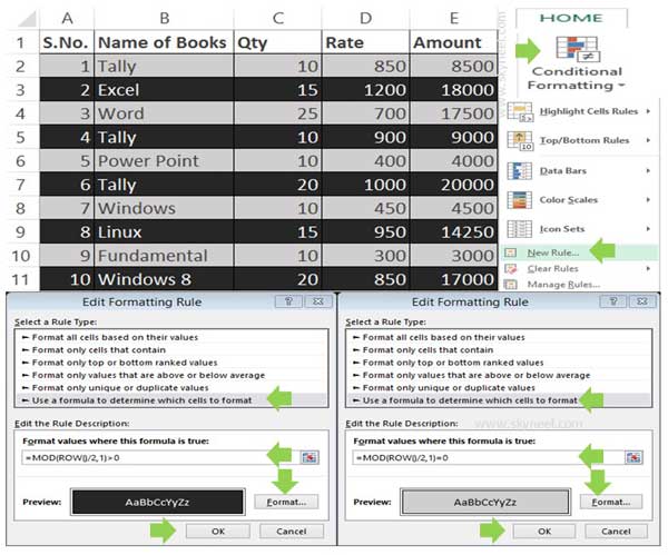
Sometime we you are working on large worksheet you need to automatically apply alternate color shading between rows in Excel. If you do this job manually then it will take lot of time. Conditional formatting allows you to quickly apply alternate color shading between rows in Excel.
During working on active worksheet you can use Conditional Formatting feature to decorate the sheet. Conditional Formatting allows you to apply different kind of formatting on selected range of cells in active sheet. You can apply background colors, borders, shading, fonts style that match certain given conditions.
Must Read: How to Sum or Count cells based on background color in Excel
How to Apply Alternate Color Shading Between Rows in Excel
There is lot of ways from which you can apply alternate color shading between rows in Excel. In this guide we have to discuss an this issue with the help of Conditional Formatting features. There are lot of situations in which you can use conditional formatting features on active worksheet. If you need to apply alternate color shading between rows in Excel then you have to take given simple steps.

Step 1: Create the following table on which you want to apply alternate color shading between rows in Excel.
Step 2: Select the range of cells on which you want to apply alternate color shading between rows in active worksheet.You can use Shift + Arrow key to select specific area of continuous range of cells. If you want to apply alternate color shading between rows in whole worksheet then press Ctrl+A shortcut key.
Step 3: Click on the Home Tab > Conditional Formatting > Click on the New Rule… option.
Must Read: 3 Ways to quickly find duplicate values in Excel
Step 4: Select “Use a formula to determine which cells to format” option in Rule type. Now type the following function in edit the Rule Description box =MOD(ROW()/2,1)>0. Now click on the Format button and apply required formatting as per your need. Click on the OK button to apply the first conditional rule for shading the color on selected rows.
Step 5: Just like this you can create another new rule type on selected range of cells and then apply the given formula =MOD(ROW()/2,1)=0. Apply the required formatting as per your need with the help of Format button. Click OK button to apply alternate color between rows in Excel.
Note: If you want to make any changes on selected conditional formatting then click on the Manage Rules… option. You can also remove the conditional formatting on selected range of cells from Clear Rules > now, click on the “Clear Rules from Selected Cells…“. If you want to quickly remove conditional formatting from entire worksheet then you have to choose “Clear Rules from Entire Worksheet…“.
Must Read: Quickly delete blank rows and columns in MS Excel
I hope this guide is useful for all those guys who want to apply alternate color between rows in Excel. Conditional formatting gives a decorative look on your active worksheet. If you have any suggestion regarding this guide then please write us in the comment box. Thanks to all.
💬 Loading comments...