Goal Seek feature in Excel is an important part of What-If-Analysis. it is an important feature of Excel which allows you how to one value in the formula impacts to other cell value. Goal Seek is the best tool used to find the result by adjusting an input value. There are lot of situation in which you can use Goal Seek feature during preparing different kind of reports. If you have more than one variable values and you want to change the final result value but want to apply effect only for one cell.
Must Read: How to Age calculation From Date of Birth – MS EXCEL
In that situation you must have to use Goal Seek feature in Excel sheet to find the answer of your query. There are lot of interesting and useful feature of Excel which allows you to solve complex calculations.
What if Analysis is an important tool of Excel. What-if-Analysis is a process which allows you to changing the values in the given cells and watch the effect on resulted value cell. What-if-Analysis has four important parts – Goal Seek, Solver, Data Table and Scenario Manager. In this guide we have to discuss about the beauty of Goal Seek feature in Excel to find the answer of your query.
Goal Seek is used to change the single value and view the impact for other values. It is an important part of What-If-analysis. You can change single value and view the impact on the resulted value. Goal Seek feature allows you to change single variable value while solver allows you to change more than one variable values and view the impact for others. Data tables also an important part of What-If-Analysis. You can not create the one input data table but also create two input data table in MS Excel.
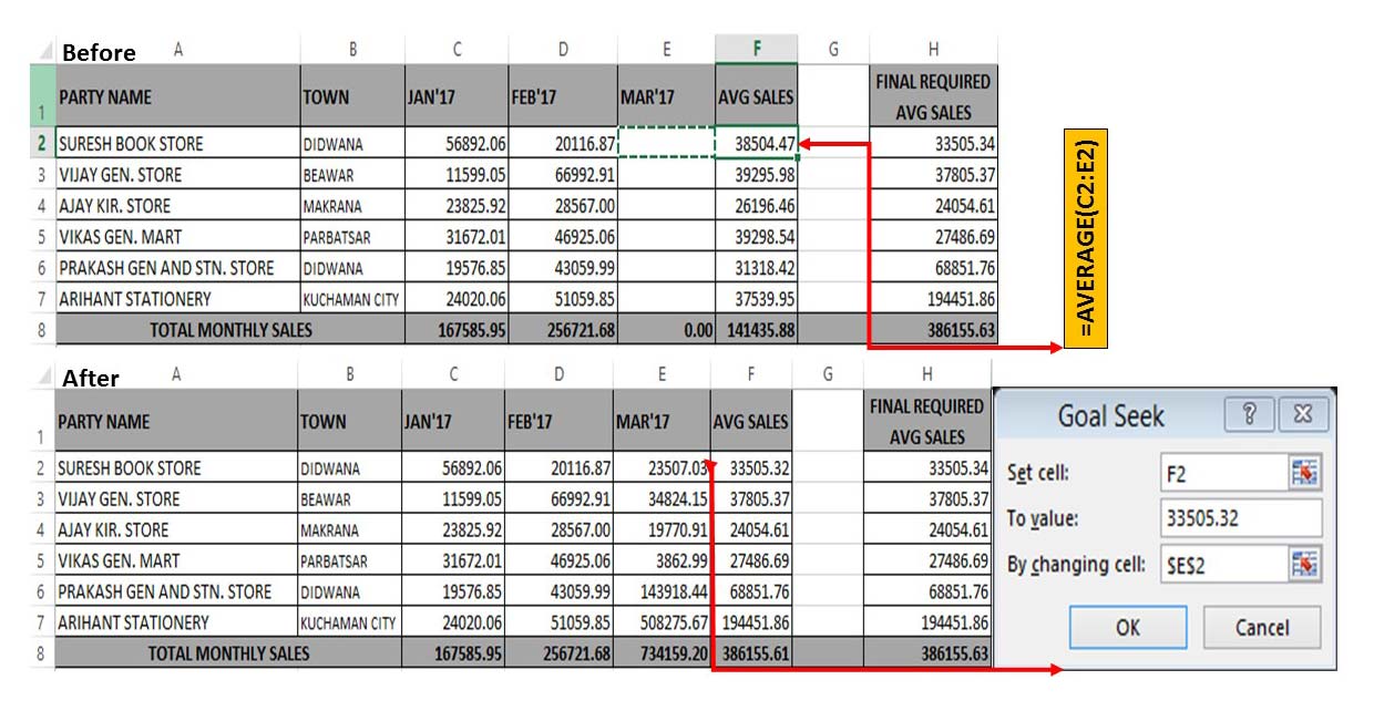
For eg: If you have a large worksheet in which you have different columns like party-name, town and two month sales amount. Now you want to calculate the avg sales amount but third month value is still missing. Top management share party-wise three month required average sales value. Now you have an query how to use Goal seek feature to calculate the third month party-wise sales amount which match the given avg sales.
Beauty of Goal Seek feature in Excel to Find the Answer
In that situation if you want to get the exact answer of your query then you must have to use Goal seek feature in Excel.

Step 1: Create the following worksheet to watch the beauty of Goal seek feature in Excel to find the answer.
Must Read: Using PPMT Function Creating a Mortgage Calculator in Excel
Step 2: Calculate the average sales amount by typing the following given formula in cell F2 =AVERAGE(C2:E2). Copy the formula to rest of the cell either from fill handle or from copy and paste command.
Step 3: In H column you will get party-wise final required average sales but March’17 detail is missing. In that situation you have to use Goal Seek feature to get the March’17 detail which match the final required average sales. To do this job select the the cell F2 and open Goal Seek feature from Data Tab > What-if-Analysis > Goal Seek….
Step 4: In Goal Seek dialog box fill the required information
Set cell: F2 (Select formula cell in which result is effected)
To value: 33505.32 (Value which you want to view as a final result)
By changing cell: $E$2 (Cell address in which change are done)
finally click on the OK button. Now apply the same procedure for rest of the cells to get the result.
I hope after reading this guide you can easily use Goal Seek feature in Excel sheet. If you have any suggestion regarding this guide then please write us via comment box. Thanks to all.
💬 Loading comments...