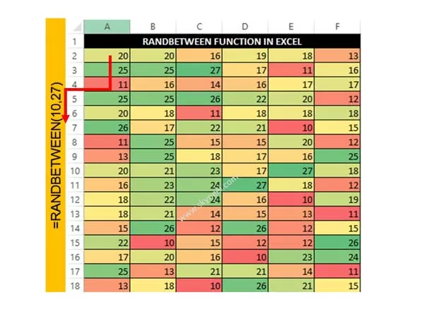
The Excel RANDBETWEEN function is very popular function which is located in Math & Trig category. Microsoft Excel RANDBETWEEN function is used to returns a random number between the number you specify. This function returns a random number which is between a bottom and top range. The RANDBETWEEN function in Excel returns a unique random number every time when your spreadsheet recalculates with the help of F9 key.
Also see:
- How to download Voter ID Card in Smartphone
- What is E-PASSPORT, Its FEATURES and How to Apply E-Passport
Must Read: How to use Countif function with wildcards in Excel
The RANDBETWEEN function is important built-in function in Excel. The RANDBETWEEN function in Excel is found in Math and Trig category. You can use this function as a worksheet function in active worksheet. RANDBETWEEN function recalculates random number when you opened any worksheet or making any changes in active worksheet. This function is used to generate a random number from lower to largest value. This number is recalculate when you have to do any kind of changes in active worksheet.
Syntax of RANDBETWEEN
RANDBETWEEN (bottom, top)
Must Read:
- How to Check the Exact Time When Your WhatsApp Message Read
- MS Excel: How to Count values in MIS report PivotTable
Bottom – It is required integer number which representing the lower value of the range.
Top – This is another required integer which representing the largest value of the range.
How to use the RANDBETWEEN Function in Excel
If you want to get a random integer number between 10 to 27 in that situation you have to use RANDBETWEEN function in Excel. You have to take few given simple steps to get the result in active worksheet.
Must Read: Using PPMT Function Creating a Mortgage Calculator in Excel

Step 1: Open an existing worksheet or create a new worksheet in which you want to use RANDBETWEEN Function.
Step 2: Type the following function in Cell A2 =RANDBETWEEN(10,27) and press enter. Now drag this function with the help of Fill Handle button as per your need.
You can drag this function either top to bottom or left to right as per your requirement.
Must Read: How to sort data based on color in Excel
Step 3: After getting the list of random number you can also apply Conditional Formatting on selected range of cell. Conditional Formatting give attractive look of your random number list.
If you want to refresh this list then you have to Press F9 Function key. After pressing this key all random numbers recalculate. I hope this guide helps you to easily learn how to use RANDBETWEEN function. If you have any suggestion or doubt then let me know by sharing your query in comment box.
💬 Loading comments...