Most of the person want to know how to return multiple corresponding values for one lookup value in Excel. VLookup in Excel allows you to quickly return multiple items with-in a short period. VLookup is very powerful and important function of Excel.
Also see:
- How to download Voter ID Card in Smartphone
- What is E-PASSPORT, Its FEATURES and How to Apply E-Passport
It is used to search for a value in first column of given table array. This function return the resulted value in the same row from another column in active table array. VLookup function located in the Lookup and Reference category of Microsoft Excel. There are a large variety of inbuilt function in Excel. VLookup is one of the most important function which is used to search values which match the specific given condition. You can also use VLookup in Excel to search duplicate values, apply VLookup with more than one criteria and many more situations.
Must Read: Advanced VLookup trick with Data Validation in Excel
Syntax of VLookup function
The Microsoft Excel VLookup function searches a value in the extreme left column of the table or array. This function provide the value in the same row which is based on the index number.
VLookup (lookup_value, table_array, col_index_num, [range])
Must Read:
Note: Before using the VLookup function, first you need to arrange first column of a table or array in the ascending order, otherwise VLookup function is not able to provide the accurate result.
Lookup_value: Lookup value is the value to be searched in the extreme first column of table or an array.
Table_array: Two or more columns of data. Give cell reference of a range / range name.
Col_index_num: It is the number which is used to be searched value must be returned.
Range_lookup: It is an options part of this function. There are two options available in this part.
TRUE: Appropriate Match. If first column sorted in ascending order then it works properly. If your table does not have ascending order then it displays wrong result.
False: Exact Match: VLookup by default check only on exact match method.
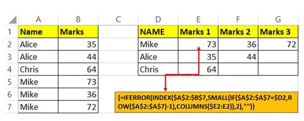
For E.g: If you have students marks in a worksheet but there are few students names are duplicate in that situation you want to lookup each student marks and set them in different columns. In other words you want to return multiple corresponding values for one lookup value in Excel. In that situation you must have to use VLookup function in Excel.
How to Return Multiple Items with VLookup in Excel
 Step 1: Prepare the following given table in your active worksheet. Now you can check that few student names are duplicate and you want to set them in E, F and G column in largest to smallest numbers.
Must Read: Slicers in Excel used to Filter PivotTable Data
Step 2: Take the cursor on cell E2 and type the given function in cell E2 =IFERROR(INDEX($A$2:$B$7,SMALL(IF($A$2:$A$7=$D2,ROW($A$2:$A$7)-1),COLUMNS($E2:E2)),2),””) now press Ctrl+Shift+Enter shortcut key.
Step 3: Copy the cell E2 formula for rest of the cells with the help of fill handle feature in Excel.
I hope after reading this guide you can easily return multiple items with VLookup in Excel sheet. Write us your suggestion in comment box. Thanks to all.
💬 Loading comments...