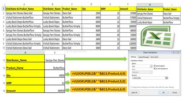
VLookup is an important lookup function which allows you to lookup specified value as per the given condition. Data validation allows you to apply different set of rules on selected range of cells. In this guide we have to discuss advanced VLookup trick with Data Validation in Excel. You can use VLookup function along with Data Validation to solve complex condition and get the exact result.
Also see:
- How to download Voter ID Card in Smartphone
- What is E-PASSPORT, Its FEATURES and How to Apply E-Passport
Sometime we need to apply VLookup function along with Data Validation command in active worksheet. It is an advanced VLookup trick used with data validation in Excel.
Must Read: Calculating Person’s current age using DATEDIF in Excel
Data Validation in Excel
Data Validation is an important feature of Excel. It is used to prevent the invalid data being entered into the cell. It is used for naming the range of selected cell contents, create drop down list, apply restriction as per your need on selected cells and many more.
VLookup Function in Excel
VLookup is an important lookup function. This function is located Lookup and Reference category of Microsoft Excel. You can use VLookup function to search specific value in extreme left column of active table_array. After that you will get the resulted value in the same row which is based on the index number.
Must Read:
- Beauty of Goal Seek feature in Excel to Find the Answer
- How to quickly remove all blank cells in MS Excel
Syntax of VLookup Function: VLookup (lookup_value, table_array, col_index_num, [range])
Note: Before start the lookup process you must have to arrange first column of a table or array in the ascending order, otherwise VLookup function is not able to provide the accurate result.
Lookup_value: Lookup value is the value to be searched in the extreme first column of table or an array.
Table_array: Two or more columns of data. Give cell reference of a range / range name.
Col_index_num: The column index_number in the table from which the searched value must be returned.
Range_lookup: It is an options part of this function. There are two options available in this part.
TRUE: Appropriate Match: This option work properly when first column of your table is sorted in ascending order only. If your table does not have ascending order then it displays wrong result.
False: Exact Match: VLookup by default check only on exact match method.
Advanced VLookup trick with Data Validation in Excel
If you have more than one criteria then you have to use advanced VLookup function in Microsoft Excel. You have to take few given simple steps to use advanced VLookup trick with data validation in Excel.

Step 1: Create the given table to start the advanced VLookup trick with Data Validation process in Excel. Now, Select the range from A2:F10 and set the range name “Product” from the Name box.
Must Read: Latest VLookup trick to search with more than one criteria in Excel
Step 2: If you don’t want to type distributor name then you must have to use Data Validation command. Data validation command allows you to create the drop down list of all selected Distributor name. Just like you can also create Product_Name list with the help of Data validation command in Excel.
Step 3: To lookup the product quantity of active distributor name you must have to type the following VLookup function in cell B14 =VLOOKUP(B12&” “&B13,Product,4,0).
To find out the MRP of active distributor and product, you have to type the following VLookup function in cell B15 =VLOOKUP(B12&” “&B13,Product,4,0).
To view the Amount of active distributor and product, you have to type following VLookup function in cell B16 =VLOOKUP(B12&” “&B13,Product,6,0).
I hope after reading advanced VLookup trick with Data Validation in Excel trick solved your lot of issues. If you have any suggestion regarding this guide than please write us in the comment box. Thanks to all.
💬 Loading comments...