Most of the person want to become an Excel expert and they need more practice on different functions. In this guide we have to discuss how to use VLookup and SUM function to get the total for multiple columns in Excel sheet. During preparing the MIS reports you must have to use VLookup function to search the specific value.
Must Read: How to use Advance Backward VLookup in Reverse Order in Excel
Sometime you must have to get the total for more than one columns numerical value which is based on the lookup value. It’s not easy task for the Excel user but if you have better command then you can easily use VLookup to get values for multiple columns.
During working on a large worksheet or an array you have to search and get the total of all those values values which meet the condition you specify in the same or other worksheet. In that situation you must have to get proper knowledge of advanced VLookup
function which allows you to get the result of your query.
For eg: If you have a large worksheet data or an array. Now you want to get the total of more than one state quantity which is based on any specific month. You can use VLookup and SUM function together to get the total for multiple columns.
How to use VLookup and Sum function to get total for Multiple columns
Sometime you need to create a summary file in which you want to get the total for multiple columns which match the given condition using VLookup function. To do this job you have
to take following given steps, have a look.

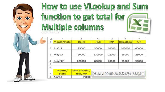
Step 1: Create the following table in same or other worksheet which is your source data. Now create a new worksheet to start the process of VLookup and SUM function together to get the total for multiple columns.
Must Read: How to Return Multiple Items with VLookup in Excel
Step 2: Type the given formula in cell B8 =VLOOKUP(A8,$A$2:$F$4,{2,3,4},0) and press Ctrl+Shift+Enter shortcut key in Excel sheet.
Now you will get first second column value as a result. If you want to get the total of qty of three states like Delhi, J&K, MP, then update the formula in cell B8 =SUM(VLOOKUP(A8,$A$2:$F$4,{2,3,4},0)). Now press Ctrl+Shift+Enter shortcut key to get the total of three states qty. This quantity is based on the lookup value with the help of VLookup and SUM function.
You can check we have to use an array {2,3,4} in the VLookup function as a third argument. This argument allows you to to get the total of lookup values of column 2,3 and 4. To convert a simple function in an array formula then you must have to press Ctrl+Shift+Enter shortcut key. Now you can watch that Excel put curly { } braces at the start and end point of your formula.
I hope after reading this guide you can easily use VLookup and Sum function in Excel. You can use them together to get the total for Multiple columns numeric values. If you have any query or suggestion regarding this guide then please write us in the comment box. Thanks to all.
💬 Loading comments...