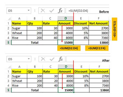
During working on excel sheet, sometime you don’t want to show applied formulas and also lock the active worksheet. In this tutorial, will discuss how to lock and hide the formula in Excel worksheet so that applied formula don’t show in the formula bar. This tutorial very useful for all those excel users who want to know about quickly lock and hide the formulas in active worksheet.
Must Read: How to Add and Use Camera in Excel Quick Access Toolbar
All we know after applying any formula, Excel will show the result in active cell. When you select the active cell in which formula applied, automatically shown in the formula bar. Formula bar is very useful and important part of Excel, which allows you to select, edit, delete and copy the formula. Normally it’s not easy to do this job for normal excel users. But this tutorial helps you how to easily and quickly lock and hide the formula in Excel worksheet.
How to lock and hide formula in Excel
If you want to preventing the formula from being showing in the formula bar, in that situation you have to take given easy steps which helps you to hide the formula in Excel worksheet.

Step 1: Open the worksheet in which you want to hide the formula.
Must Read: Insert a blank Row between existing each Rows of data in Excel
Step 2: Select whole data in active worksheet. To select the sheet either use Shift+Arrow keys or Press Ctrl+A shortcut key. You can use given excel shortcut keys to quickly select the range in active worksheet.
Step 3: Open Format Cell dialog box by pressing Ctrl+1 shortcut key. You can press Ctrl+Shift+F excel shortcut key to quickly open the Format cell dialogue box. You can also click on the Home tab and then click of Number dialogue box launcher button. Now click on the Protection tab and turn off Locked option.
Step 4: Open Go To dialog box Home > Find & Select > Go To Special option or Press Ctrl+G shortcut key > click on the Special button. Now, turn on Formula option and check all sub option like “Numbers, Text, Logical and Errors”.
Step 5: Again open Format Cell dialog box > Go to Protection tab > turn on both “Locked” and “Hidden” option and press OK button.
Must Read: How to Group and Ungroup of Excel Pivot Table Data
Step 6: Now protect the active sheet by from Review > Protect Sheet option. Here you have to turn on given two option and apply the password.
“Select locked cells”
“Select Unlocked cells”
Step 7: Now, you can check applied formula from all the cells hiding from active worksheet.
How to apply password protection on non continuous cells in Excel
Excel is an important application software which is widely used by billion of users around the world. By default password protection applied on whole worksheet. But if you need to apply password protection on particular non continuous cells. In this guide we have to discuss how to apply password protection on non continuous cells in Excel.
Sometime during working on a large worksheet data you need to protect few selected range of cells with the password. After applying the password nobody make changes in your protected cells of any worksheet.
Must Read: How to switch or flip name in Excel
How to select cells, range of cells, row or columns in Excel
Excel allows you to quickly select non-adjacent cells in or range of cells in Excel. There are lot of ways from which you can easily and quickly select more than one continuous or non continuous cells in active worksheet. Mouse and Keyboard play an important role during selecting a large worksheet data. Excel allows you to quickly select cells, range of cells, row or columns in Excel sheet.
💬 Loading comments...