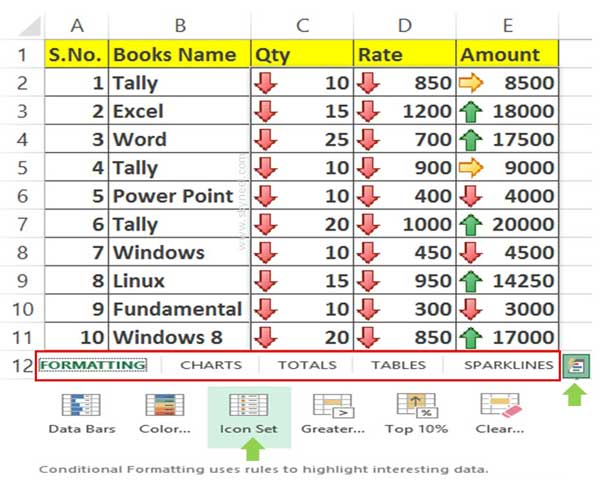
Quick analysis is an important tool which allows you to quickly analyze your selected range of cells. Quick analysis feature in Excel not only analyze your data but also prepare chart, conditional formatting, apply different functions and many more.
Also see:
- How to download Voter ID Card in Smartphone
- What is E-PASSPORT, Its FEATURES and How to Apply E-Passport
All we know Excel has lot of interesting and useful features which are very useful for us. During working on the Excel, sometime you have to take lot of time to do any job. But if you have proper knowledge about the complete features then your working time will be reduced during working on Excel. Quick analysis is an important tool which allows you to apply formula, color coding, charts during analysis of your selected range of data.
Must Read: How to Age calculation From Date of Birth – MS EXCEL
Steps How to Use Latest Quick Analysis Feature in Excel
Excel is an important utility application software. There are lot of extra ordinary features which helps the users to get the quick result and save the working time. Quick analysis feature in Excel allows you to quickly check your selected range of cells. If you want to use quick analysis feature in active worksheet then you have to take few given simple steps, have a look.

Must Read:
- Remove spaces with Data Validation in MS Excel
- Disk Partition: How to Partition of Hard Disk by easy steps
Step 1: Select the range of cell in which you want to apply quick analysis feature in Excel. After selecting the range you can see quick analysis icon at the right bottom part in active worksheet.
Step 2: Just click on the icon, now you will get Formatting, Charts, Totals, Tables & Sparklines. Each group has different options, you can choose any required option as per your need.
Formatting: You can easily apply required conditional formatting to highlighted the required data on the selected range of cells.
Charts: If you want to prepare graphical presentation of your selected numerical data then you have to use this feature.
Totals: Use this feature to quickly get sum, avg, count, calculate percentage on selected range of cells.
Must Read: How to use Flash Fill or Auto Fill command in Excel
Tables: If you want to get summarize data, apply sorting or filtering. You can also create pivot table on selected range of cells with this option.
Sparklines: These are mini chart and it is placed in a single cell. If you want to prepare mini charts of selected range of cells then you have to use sparklines.
I hope after reading this guide you can easily understand how to Use latest Quick Analysis feature in Excel. If you need smart working then you must have to know about these feature. If you have any suggestion regarding this guide then please write us in the comment box. Thanks to all.
💬 Loading comments...